Hongxu Xu

PhD Student (May 2025 – Present)
Supervised by Prof. Chengnian Sun
Cheriton School of Computer Science
University of Waterloo, Canada
B.Sc. in Computer Science (Sep 2014 – Jun 2018)
Beijing Normal University, China
Research Interests
- Software Engineering
- Programming Languages
with a focus on compiler optimizations, software testing, and formal verification.
Socials
- GitHub: https://github.com/xuhongxu96
- Google Scholar: https://scholar.google.com/citations?user=kmb2dP8AAAAJ
- LinkedIn: https://www.linkedin.com/in/xuhongxu/
- Email: h4️⃣4️⃣5️⃣xu 🌀 uwaterloo.ca
If you’d like to hear more about my thoughts and life, consider following me on:

-
Substack: https://hongxuxu.substack.com/ (English only)
Subscribe to my newsletter on Substack to get my latest updates. -
微信公众号: xuhongxu_it (Chinese only)
Scan the QR code on the right to follow my WeChat Official Account.
扫描右侧二维码 关注我的微信公众号。
Misc.
- Chinese Name: 许宏旭
- Literally means “宏: Great 旭: Rising Sun”
- Pronunciation:
Hong-shioo(IPA:[xʊŋ ɕy])
Publications
Papers
ISSTA'26Automated Dependency Optimization for Artifact-Based Build Systems
Hongxu Xu, Zhenyang Xu, Shane McIntosh, Chengnian SunASPLOS'26LPO: Discovering Missed Peephole Optimizations with Large Language Models
Zhenyang Xu, Hongxu Xu (Co-First), Yongqiang Tian, Xintong Zhou, Chengnian Sun
Books
Feb 2024CMake构建实战:项目开发卷 (CMake Build Practice: Project Development Volume)
Published by 人民邮电出版社 (Posts & Telecom Press, China)
Produced by 异步图书 (epubit)
Experience
PhD Student (May 2025 – Present)
Supervised by Prof. Chengnian Sun
Cheriton School of Computer Science
University of Waterloo, Canada
Senior SDE (Sep 2022 – Mar 2025)
Seed/Data Speech Team
ByteDance, Shanghai, China
Led the development of the Text-to-Speech engine and contributed to the Doubao AI assistant application.
SDE-2 (Aug 2021 – Sep 2022)
MSAI Team
Microsoft STC-Asia, Suzhou, China
Led the development of Microsoft WordBreaker and initiated a modern NLP toolkit for Office 365.
SDE (Jul 2018 – Aug 2021)
MSAI Team
Microsoft STC-Asia
Beijing, China (Relocated to Suzhou, Jiangsu, China in May 2019)
Worked on Microsoft WordBreaker.
Short-Term Contributor (Nov 2020 – Jan 2021)
Windows APS Team (temporary assignment)
Microsoft STC-Asia, Suzhou, China
Contributed to the formation of the new team and Windows 11 application development (MS Calculator).
B.Sc. in Computer Science (Sep 2014 – Jun 2018)
Beijing Normal University, China
SDE Intern (Jul 2017 – Dec 2017)
Bing Search Relevance Team
Microsoft STC-Asia, Beijing, China
Worked on answer triggering models for Bing Search.
Awards
- Outstanding Graduate, Beijing Normal University, 2018
- Top Ten Volunteer, Beijing Normal University, 2015
- First Prize, National Olympiad in Informatics in Provinces (NOIP), 2013
Teaching
Note
IA: Instructional ApprenticeTA: Teaching Assistant
IA, CS 246 - Object-Oriented Software Development, Spring 2026IA, CS 136L - Tools and Techniques for Software Development, Winter 2026IA, CS 246 - Object-Oriented Software Development, Fall 2025TA, CS 246 - Object-Oriented Software Development, Spring 2025
My Thoughts and Life
Note
I share technical content on this website, including course notes, projects, and research.
For more personal thoughts and life updates, please check out my Substack newsletter and WeChat Official Account below.
Tip
Follow me on Substack and WeChat!
Substack: https://hongxuxu.substack.com/ (English only) Subscribe to my newsletter on Substack to get my latest updates.
微信公众号: xuhongxu_it (Chinese only) Scan the QR code on the right to follow my WeChat Official Account. 扫描右侧二维码 关注我的微信公众号。
Selected Substack Posts
My First ASPLOS - The Journey and the Learning
My 2025
G1 Pain Points
Useful Resources
Compiler
Formal Methods
Rust
InstCombine Debugger
https://xuhongxu.com/instcombine-instrumentor/
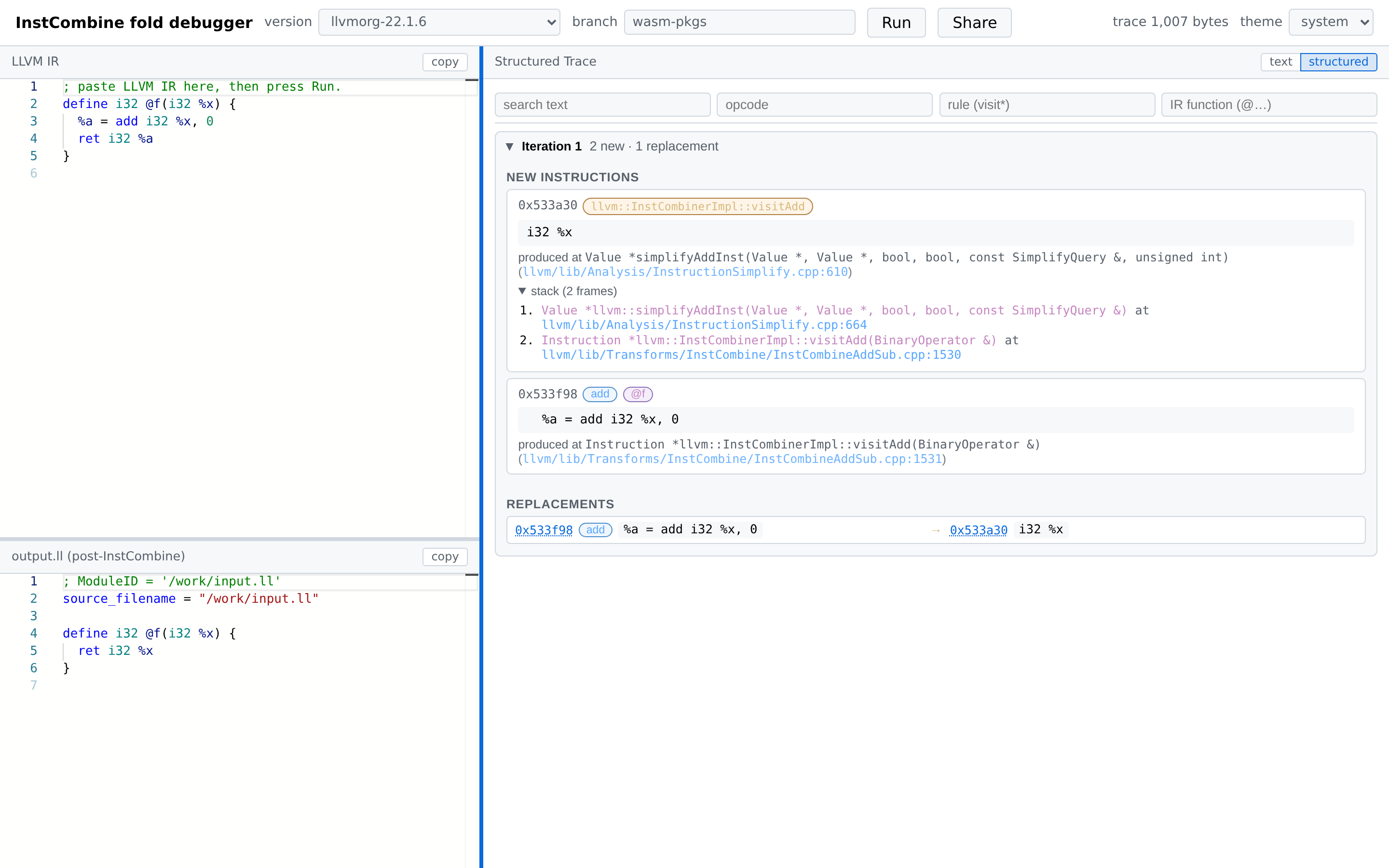
See Every Rewrite InstCombine Makes — In Your Browser
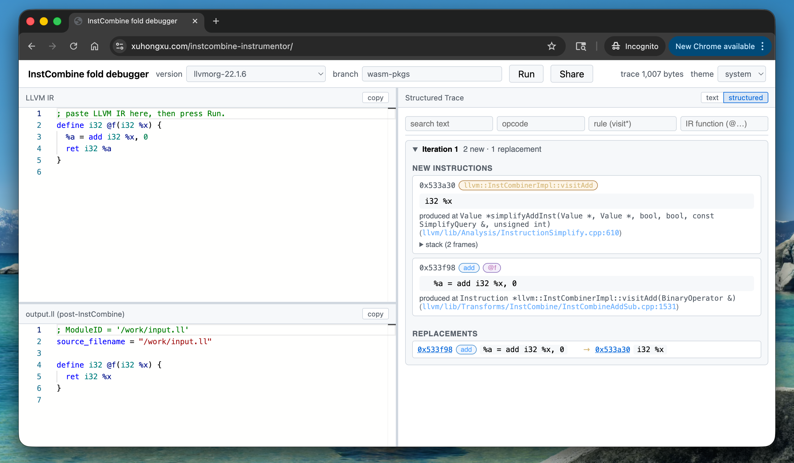
LLVM’s InstCombine is the workhorse peephole pass: it rewrites IR thousands of times per compile, but when one of those rewrites surprises you, finding out which rule fired, why, and on what value usually means a local LLVM build, printf debugging, and a lot of patience.
Recommended Reading:
InstCombine Instrumentor is a browser-based debugger that skips all of that.
Paste IR, hit run, and see exactly what InstCombine did to it — instruction by instruction, iteration by iteration.
What you get
- Input IR — paste any LLVM IR .ll snippet
- Output IR — the IR module after InstCombinePass runs.
- Trace — every new
Value*created and every RAUW (ReplaceAllUsesWith) performed, grouped per fixed-point iteration.
The trace pane has two modes:
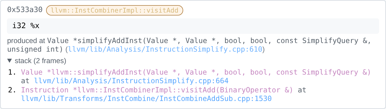
- Structured (Default) — collapsible iterations, opcode/rule/function pills, filterable by text/opcode/rule/function, with clickable cross-links between replacements. More user-friendly for interactive debugging and exploration.
- Text — each value tagged with opcode, function/BB, rule, and call-site stack. Better for bug reports and offline analysis.
Why it’s useful
- No build. It’s WebAssembly.
The wasm bundle ships with the page; no install, no checkout, no toolchain. - Pick your LLVM.
The version dropdown lists every tagged LLVM release we’ve bundled (Create a pull request to add more). Reproduce a bug against the exact version you’re targeting. - Frame-accurate traces.
Each value is captured at the call site that produced it —__FILE__:__LINE__of the wrapping call, plus the__PRETTY_FUNCTION__of the caller — so you see the rule that fired, not just the leafIRBuilderhelper. - Same trace, native or browser.
We directly patch LLVM’s InstCombine source to emit the trace, so the browser and native builds produce the same output.
Who it’s for
- Compiler engineers writing or reviewing InstCombine patches.
- LLVM contributors triaging “this rewrite looks wrong” bug reports without having to build anything.
- Anyone learning how InstCombine works — watching the fixed-point loop unfold on a small example is the fastest way to build intuition.
Examples
Tip
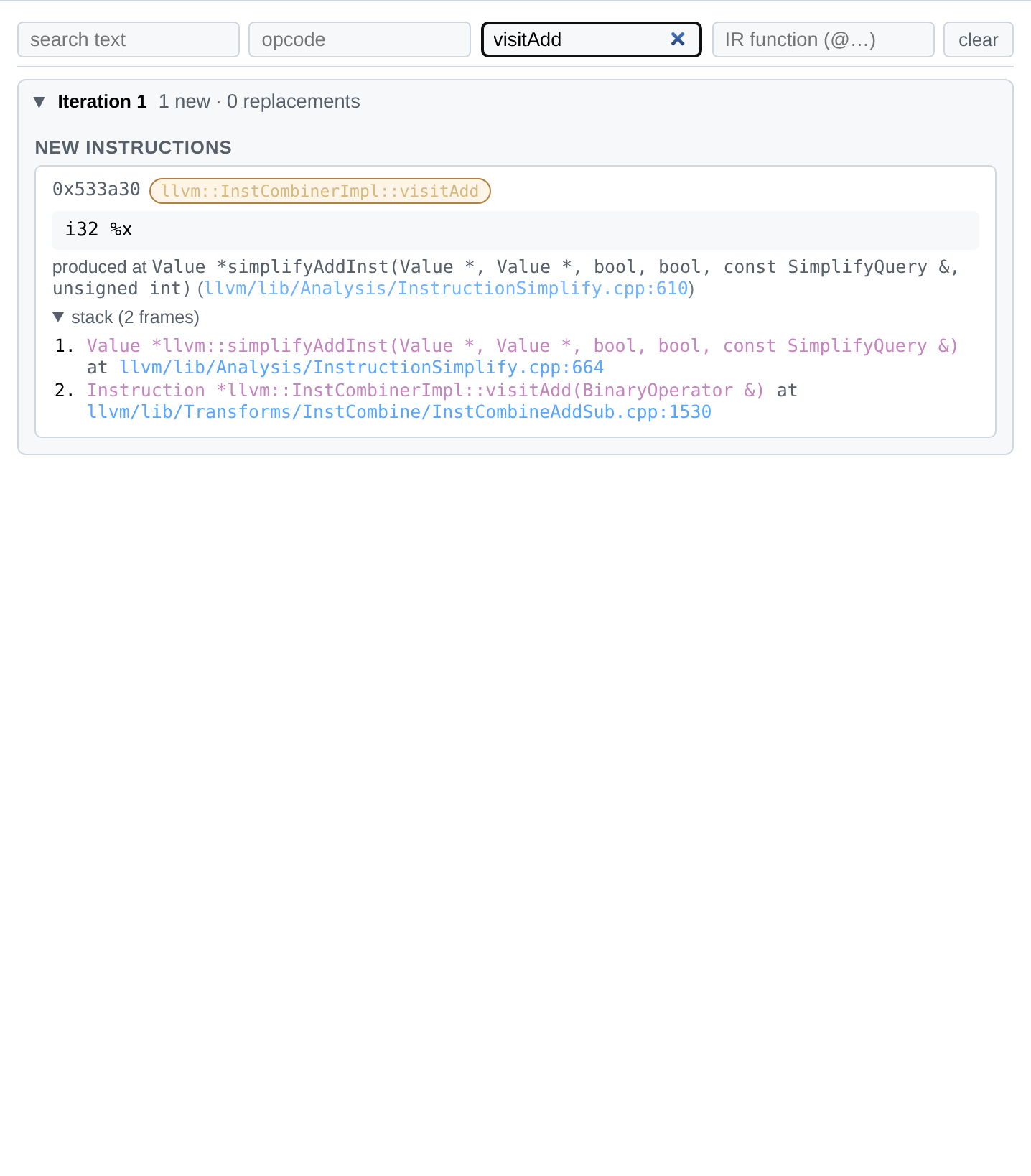
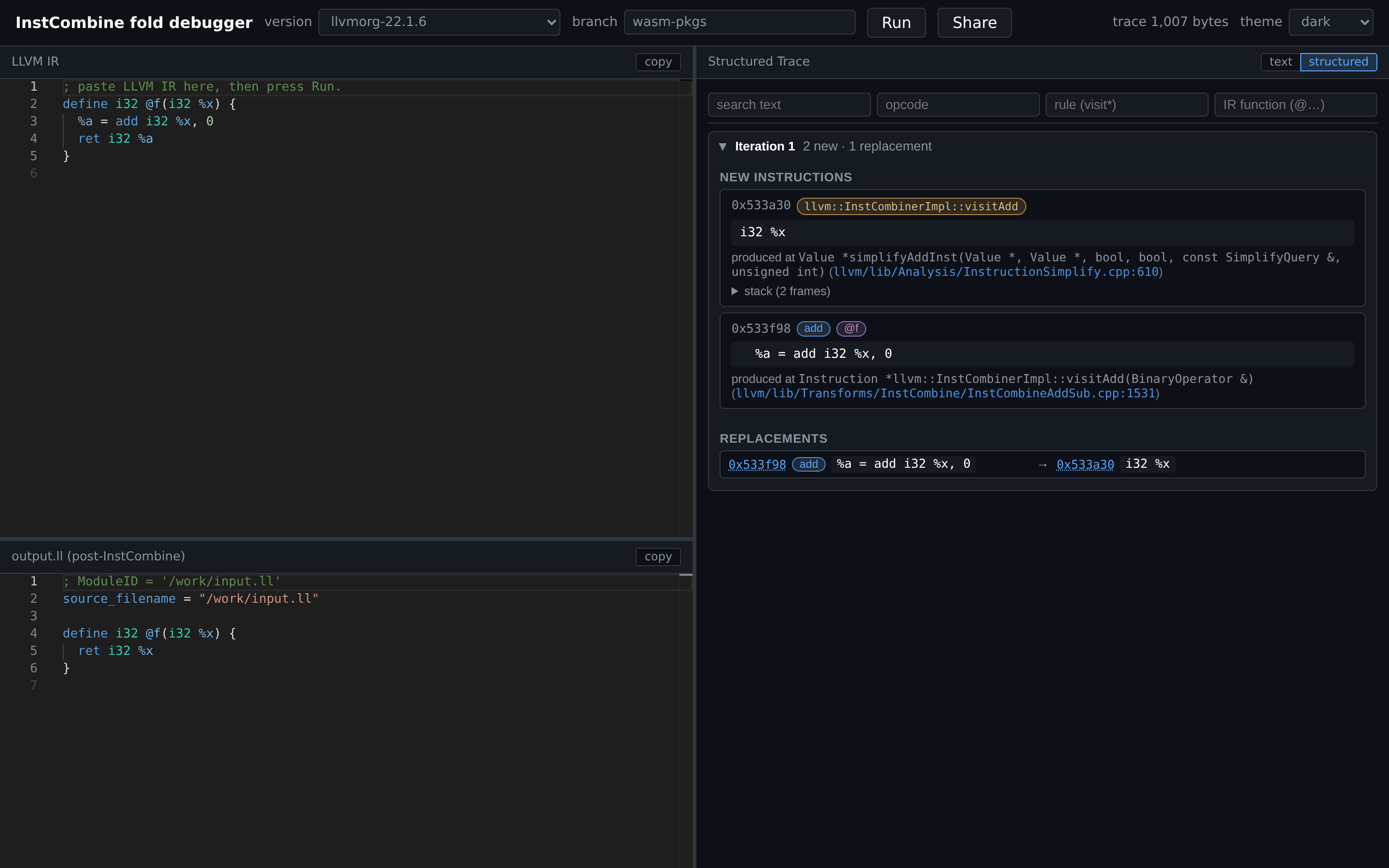
Try a tiny IR snippet first (a couple of adds with a 0 operand will do), flip to the Structured View, and watch the rules fire.
define i32 @f(i32 %x) {
  %a = add i32 %x, 0
  ret i32 %a
}
; no rewrite in LLVM 21 and earlier
define i1 @src(i8 %x) {
  %lshr = lshr i8 4, %x
  %trunc = trunc i8 %lshr to i1
  ret i1 %trunc
}
; no rewrite in LLVM 21 and earlier
define range(i32 0, 7) i32 @src(i32 %0) local_unnamed_addr #0 {
  %2 = insertelement <4 x i32> poison, i32 %0, i64 0
  %3 = shufflevector <4 x i32> %2, <4 x i32> poison, <4 x i32> zeroinitializer
  %4 = tail call i32 @llvm.vector.reduce.add.v4i32(<4 x i32> %3)
  ret i32 %4
}
Open Source
https://github.com/xuhongxu96/instcombine-instrumentor
Welcome contributions! See the README and CLAUDE.md for details.
InstCombine Fold Debugger — User Manual
A browser-based debugger for LLVM’s InstCombine pass. Paste IR, click Run, and inspect every new value, every replacement, and the call stack that produced each one — all without installing anything. Live site: https://xuhongxu.com/instcombine-instrumentor/.
This manual has two parts:
- Part I — Using the webapp for end users.
- Part II — Operating the CI for maintainers who publish new builds.
Part I — Using the webapp
1. At a glance
The window is split into three resizable panes:
| Pane | Position | Contents |
|---|---|---|
| LLVM IR | top-left | Input editor — paste or edit IR here |
| output.ll | bottom-left | Optimized IR after the pass (or driver stderr on parse errors) |
| Trace | right | Per-iteration record of new instructions and RAUW replacements |
A toolbar runs across the top with the version picker, branch picker, Run, Share, a status line, and a theme picker.
2. Toolbar

-
version — Selects which prebuilt LLVM/
InstCombinewasm bundle to run. Two groups appear in the dropdown:- Tagged releases (e.g.
llvmorg-22.1.6) — stable LLVM tags. The newest one is selected by default. - Commit snapshots (e.g.
main-260524-abc1234567ef) — daily builds tracking LLVMmain.
Selection is remembered per-browser via
localStorage, and can be preselected via?tag=…in the URL. - Tagged releases (e.g.
-
branch — Picks which GitHub branch supplies the wasm bundles. The default
wasm-pkgsis the canonical published branch. Override with?branch=…in the URL if you’ve published bundles on a fork. -
Run — Runs
InstCombineon the current IR. Disabled while a wasm bundle is loading or a previous run is in flight. -
Share — Copies a permalink to the clipboard. The link encodes the IR (compressed), the selected version, and the branch. The button shows link copied for ~1.5 s on success.
-
status — Right-aligned text:
loading manifest…,loading <tag>…,running InstCombine…,trace <N> bytes, or an error message. -
theme —
system/light/dark. Applied instantly to the whole UI and persisted across reloads.
3. Editing input IR
The LLVM IR pane is a Monaco editor with LLVM-IR syntax highlighting. It comes prefilled with a one-line sample (%a = add i32 %x, 0) so you can hit Run immediately. Paste your own IR over it, or load IR from a share link with ?ir= / ?irz= URL parameters. The copy button in the pane header copies the current contents to the clipboard.
4. Running InstCombine
Click Run. The wasm driver parses the IR, runs InstCombine as a FunctionPass, writes the optimized IR back to a virtual filesystem, and dumps the trace. The status line transitions to trace <N> bytes when the run completes.
If parsing fails, the output.ll pane switches to plaintext mode and shows the driver’s stderr — useful for diagnosing malformed IR.
5. Output IR pane
Read-only Monaco editor showing output.ll from the wasm driver. Word-wrap is off for valid IR and on for error text. The copy button copies the visible text.
6. Trace pane
The trace pane has two view modes — toggle via the text / structured segmented control in the pane header. The toggle does not persist across reloads (default is structured).
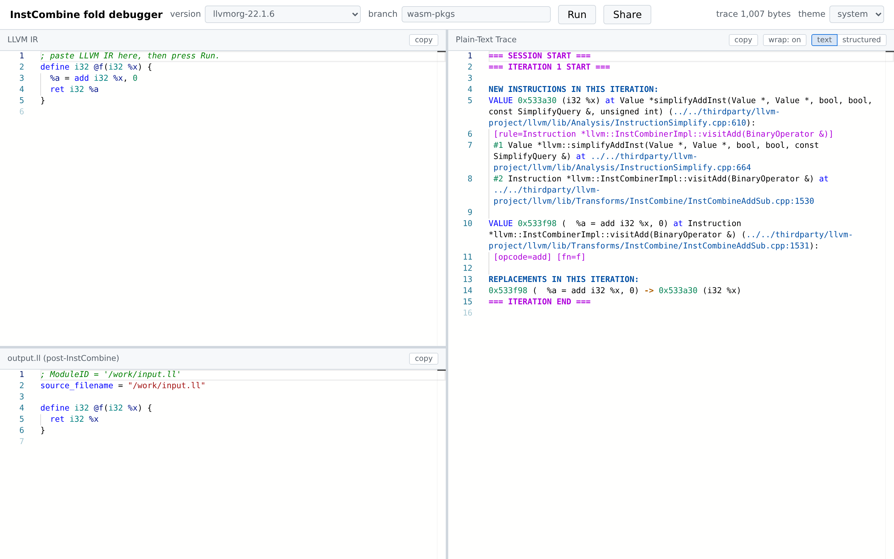
6.1 Text mode
Renders llvm_fuzz_info.txt verbatim with custom syntax highlighting for === ITERATION … markers, pointer-arrow replacements, stack frames, and source locations. A wrap toggle controls long-line wrapping; copy copies the full trace.
6.2 Structured mode
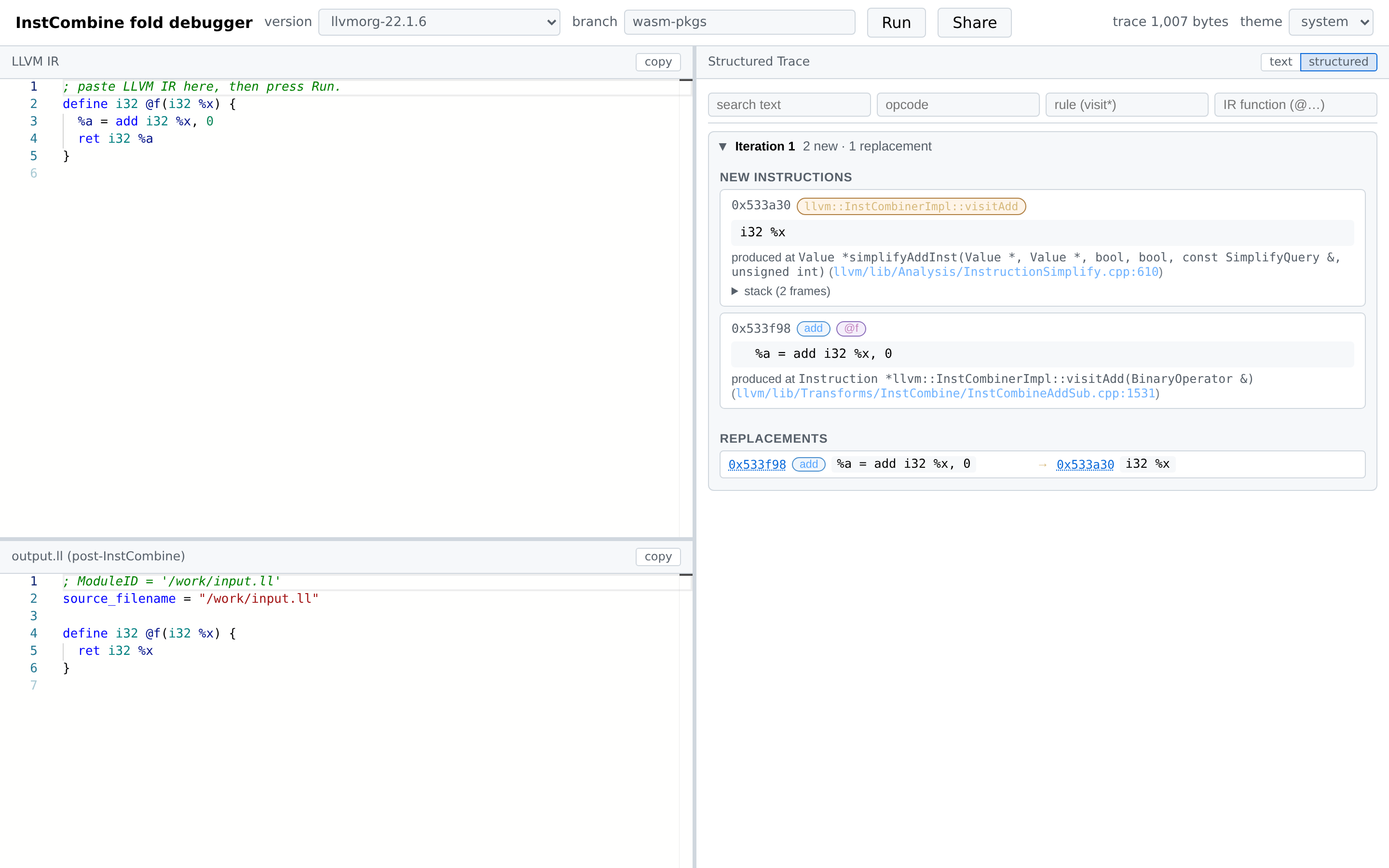
Each InstCombine fixed-point iteration is rendered as a collapsible card. Inside an iteration:
-
NEW INSTRUCTIONS — one card per
Value*produced during the iteration, showing:-
Pointer address (clickable cross-link target).
-
Pills for opcode (blue), parent function/block (purple), rule (orange — the
InstCombinevisitor that fired), and debug location (green — only when the IR carries DI metadata). -
The instruction text.
-
“produced at …” with a clickable GitHub link to the source line of the wrapping
__llvm_fuzz_record(...). -
An expandable stack showing all outer call sites:
-
-
REPLACEMENTS — every
Value::doRAUWfrom the iteration asold → new, each side showing pointer + opcode pill + IR. Pointer addresses are clickable: clicking scrolls to the matching value card and briefly flashes it.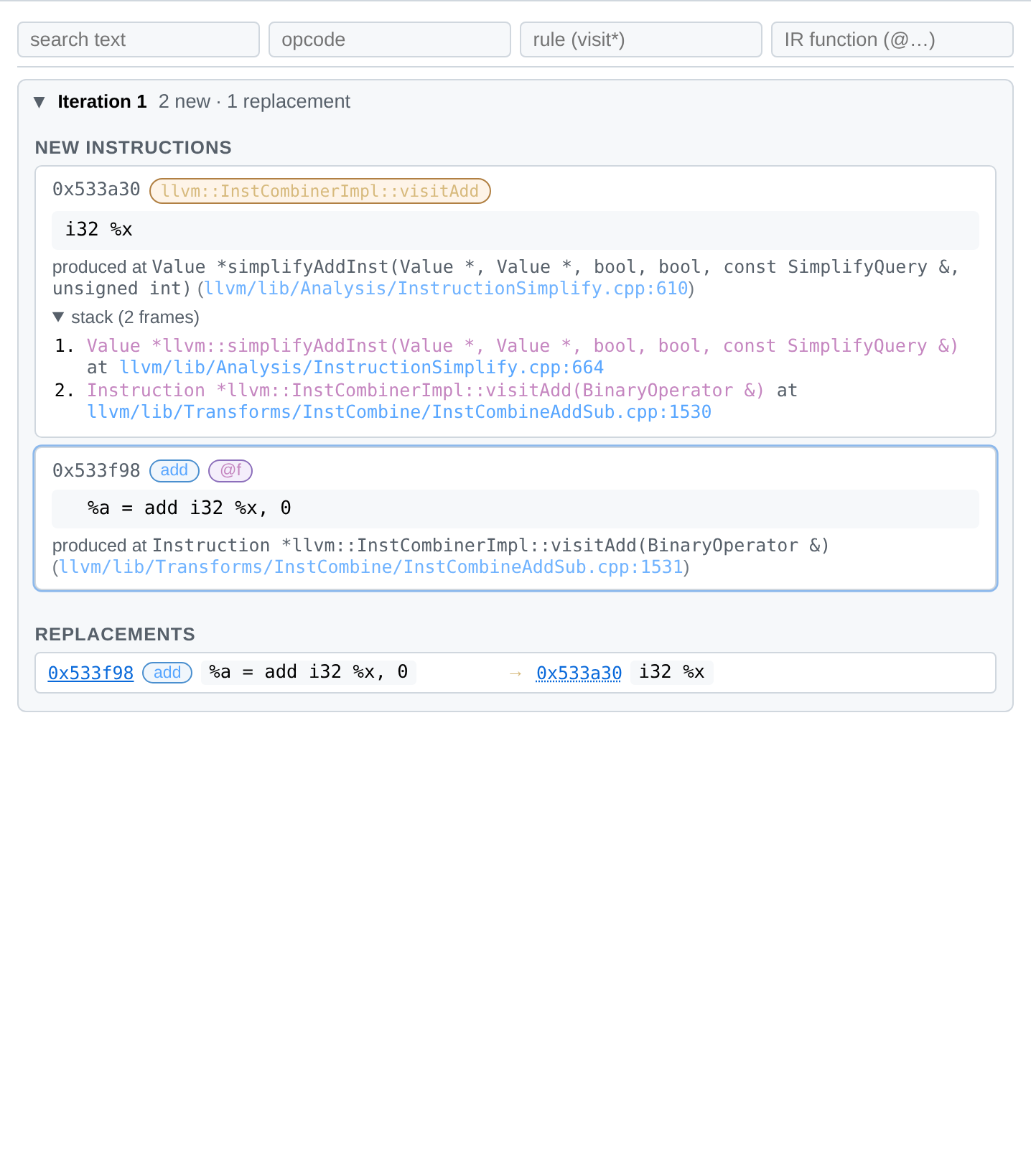
A sticky filter bar at the top of the structured view narrows the visible records live as you type. Four independent filters compose with AND semantics:
| Filter | Matches |
|---|---|
| search text | anywhere in the IR text, function name, or debug location |
| opcode | LLVM opcode (add, icmp, select, …) |
| rule (visit*) | InstCombine visitor (e.g. visitAdd) |
| IR function (@…) | the parent function the value belongs to |
A clear button appears once any filter is active.
7. Share URLs
Clicking Share copies a permalink that re-creates your current session: same IR, same version, same branch.

Supported URL parameters:
| Param | Meaning |
|---|---|
?irz=<base64url> | Modern: compressed IR (DEFLATE-raw with a small built-in dictionary). |
?ir=<base64url> | Legacy: uncompressed IR. Still accepted; produced as fallback when the browser lacks CompressionStream. |
?tag=<version> | Preselect a wasm version. |
?branch=<name> | Preselect the artifact branch. |
8. Theme & layout
Use the theme picker for system / light / dark.
All three pane boundaries are draggable. Layout is auto-saved per browser; reload restores your widths.
9. Troubleshooting
| Symptom | Cause / fix |
|---|---|
Status stuck on loading manifest… | The browser can’t reach raw.githubusercontent.com. Check ad-blockers and corporate proxies. |
Status stuck on loading <tag>… | First-time fetch of a ~30 MB wasm bundle. Subsequent loads are cached. |
| output.ll shows non-IR text | The driver couldn’t parse the input IR. The pane content is the driver’s stderr. |
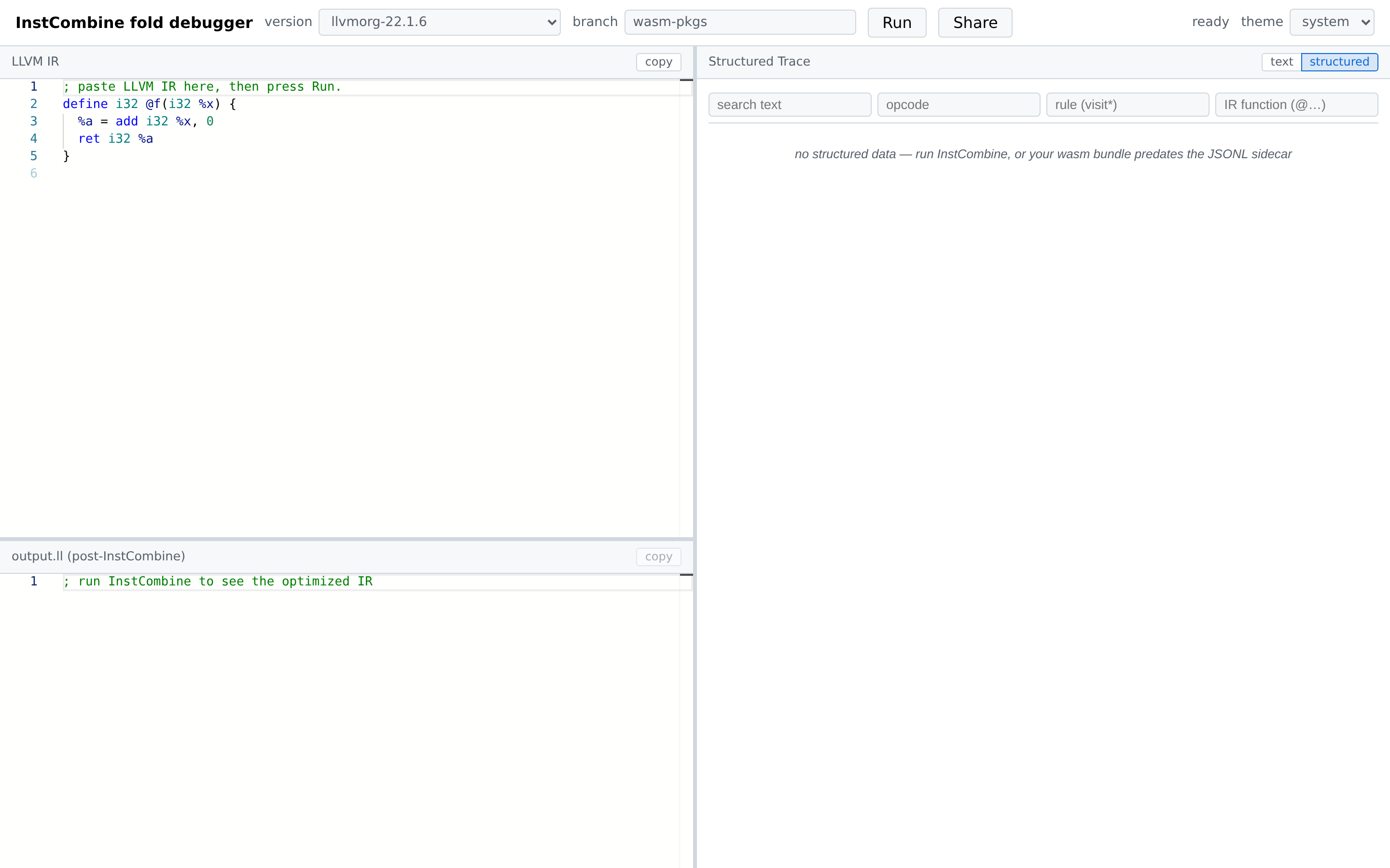
no structured data — your wasm bundle predates the JSONL sidecar | The selected bundle is older than the structured-trace feature. Pick a newer version or stay in text mode. |
| Share link doesn’t restore the IR | The link was generated by an older webapp version; the IR fragment may be truncated. |
| Pane handle won’t drag | Resize handles are 4 px wide — aim carefully; the cursor changes to col-resize / row-resize when you’re on one. |
Part II — Operating the CI
The repository ships two independent publishing tracks:
- Native
optreleases — GitHub Releases under tagrelease/<llvm-ref>, each carrying a Linux x86_64 tarball of patchedopt+llvm-symbolizer. - Wasm bundles — directories committed to the orphan
wasm-pkgsbranch, fetched at runtime by the webapp viaraw.githubusercontent.com. The webapp’s version dropdown is populated fromwasm-pkgs/manifest.json.
The two tracks share toolchain helpers (.github/scripts/shared/) but no scheduling — bumping an LLVM version in one does not implicitly bump the other.
10. Workflow map
| Workflow | Triggers | Produces |
|---|---|---|
native-build.yml | push / PR / release/* tag | Build matrix for native opt; attaches tarball to the Release on tags. |
native-release-auto.yml | Mon 05 UTC cron + workflow_dispatch | Pushes release/llvmorg-X.Y.Z for new upstream stable tags and dispatches native-build.yml. |
native-release-manual.yml | workflow_dispatch | Same as auto, but for an arbitrary LLVM tag or commit SHA. |
native-weekly-canary.yml | Mon 06 UTC cron + workflow_dispatch | Native build against LLVM main tip — pure breakage detector. No release. |
wasm-verify.yml | push / PR (wasm paths) + workflow_dispatch | Builds + smoke-tests wasm; uploads a 14-day wasm-bundle-latest artifact. Does not publish. |
wasm-publish.yml | Mon 05 UTC + every 3 days 06 UTC cron + workflow_dispatch | Builds and publishes wasm bundles to wasm-pkgs, regenerates manifest.json. |
wasm-custom-publish.yml | workflow_dispatch | Publishes a wasm bundle from a fork or alternate LLVM source URL. |
wasm-pages.yml | push to main (web paths) / PR / Mon 09 UTC cron + workflow_dispatch | Deploys the SPA to GitHub Pages; bakes the wasm-pkgs manifest URL. |
All build workflows share ccache via actions/cache@v4 keyed off llvm_commit.txt so PRs, push-to-main, and Release tags targeting the same LLVM version reuse each other’s compile cache. Helper scripts are grouped per-workflow under .github/scripts/.
11. Native opt releases
11.1 native-build.yml
Runs on every push and PR for verification, and on release/* tags it bundles opt + llvm-symbolizer into opt-llvm-<short-sha>.tar.xz and attaches it to the matching GitHub Release. No manual dispatch is needed for the normal flow — pushing a release/* tag is enough.
11.2 native-release-auto.yml
Scheduled Monday 05:00 UTC, also workflow_dispatch-able. Scans llvm/llvm-project for stable llvmorg-X.Y.Z tags that don’t yet have a matching release/<tag>, picks the newest max_tags, and for each missing tag pushes a release/<llvm-tag>, pre-creates the GitHub Release, then explicitly dispatches native-build.yml against that tag.
Inputs:
| Input | Default | Meaning |
|---|---|---|
max_tags | 1 | Maximum number of missing upstream tags to release this run. |
dry_run | false | Print the plan without pushing tags or dispatching builds. |
11.3 native-release-manual.yml
workflow_dispatch-only companion to the auto workflow. Use it to release any LLVM ref off-cron.
Inputs:
| Input | Required | Meaning |
|---|---|---|
llvm_ref | yes | Either an llvmorg-* tag or a 7–40 hex commit SHA. Branches are rejected. |
dry_run | no (false) | Print the plan without pushing or dispatching. |
Tag derivation: release/<llvm_ref> for tags; release/<YYMMDD>-<first-12-hex> for SHAs (date pulled from the GitHub commit metadata).
11.4 native-weekly-canary.yml
Scheduled Monday 06:00 UTC, also workflow_dispatch-able. Builds native opt against an LLVM ref (defaults to main) without attaching a Release. Use it to detect upstream LLVM changes that break the patcher early.
Inputs:
| Input | Default | Meaning |
|---|---|---|
llvm_ref | main | Branch, tag, or commit SHA to build. |
12. Wasm bundles
12.1 wasm-verify.yml
Push/PR (paths gated to wasm-relevant files) and workflow_dispatch. Builds the wasm bundle and runs wasm/test/smoke_wasm.mjs, then uploads a 14-day workflow artifact wasm-bundle-latest so reviewers can preview a PR build locally. No publishing to wasm-pkgs, no Release attachment, no inputs.
12.2 wasm-publish.yml
The main wasm publishing pipeline. Crons:
- Mon 05 UTC —
weekly-stablemode: publish the newest missing stable LLVM tag. - Every 3 days 06 UTC —
daily-mainmode: publish a snapshot of LLVMmainHEAD.
workflow_dispatch exposes a mode choice that selects the same logic on demand:
| Input | Default | Meaning |
|---|---|---|
mode | specific-ref | weekly-stable / daily-main / specific-ref / rebuild-existing. |
llvm_ref | '' | specific-ref only — llvmorg-* tag or 7–40 hex SHA. Comma-separated list accepted. |
max_tags | 1 | weekly-stable only — max missing stable tags to build this run. |
prune_main | 7 | daily-main only — number of main-* snapshots to retain. |
force_rebuild | false | Skip the “already on wasm-pkgs” short-circuit. |
dry_run | false | Build but don’t push to wasm-pkgs. |
rebuild-existing enumerates every published directory and rebuilds each from its corresponding LLVM ref — useful after a patch fix that affects all targets. Only the finalize job is mutex-serialized (group: wasm-pkgs), so overlapping runs can build in parallel.
12.3 wasm-custom-publish.yml
workflow_dispatch-only. Publishes a wasm bundle for an LLVM ref hosted in a fork or otherwise not on llvm/llvm-project.
Inputs:
| Input | Required | Meaning |
|---|---|---|
llvm_source_url | yes | GitHub URL of the form /tree/<branch-or-sha> or /commit/<sha>. Accepts /commits/ too. |
dry_run | no (false) | Build but do not push the artifact branch. |
Branch-backed refs are normalized to commit SHAs by .github/scripts/wasm-publish/resolve_custom_source.mjs before checkout, so subsequent rebuilds remain reproducible.
12.4 wasm-pages.yml
Builds and deploys the SPA at https://xuhongxu.com/instcombine-instrumentor/. Triggers: push to main (web paths), PR (build only — no deploy), Mon 09 UTC cron, and workflow_dispatch.
At build time web/scripts/build-manifest.mjs fetches the canonical wasm-pkgs/manifest.json and rewrites it according to a bundle mode. The webapp also reads VITE_REMOTE_MANIFEST_URL (baked into the bundle) and prefers the live manifest at runtime, so the same-origin copy is a fallback for offline / blocked-CDN users.
Inputs:
| Input | Default | Meaning |
|---|---|---|
bundle_mode | remote | remote (every version stays on raw.githubusercontent.com), hybrid (force-includes + N newest stable tags), or bundled (everything same-origin). |
bundle_count | 5 | hybrid/bundled — max auto-picked entries (force-includes are additional). |
include_commit_count | 0 | hybrid — additionally bundle the N newest main-* snapshots. |
must_bundle | '' | CSV of additional tags or SHA prefixes to force-bundle, appended to wasm-must-bundle.txt. |
13. Common maintainer recipes
- Publish wasm for a brand-new stable tag — dispatch
wasm-publish.ymlwithmode=specific-ref,llvm_ref=llvmorg-X.Y.Z. - Try a build before pushing to
wasm-pkgs— dispatchwasm-publish.ymlwithdry_run=true; the workflow artifact contains the staged outputs. - Force-bundle one version into the Pages deploy — append the version directory name to
wasm-must-bundle.txt, push tomain, then dispatchwasm-pages.ymlwithbundle_mode=hybrid. - Publish a wasm bundle from a fork — dispatch
wasm-custom-publish.ymlwith the GitHub source URL (https://github.com/<you>/<fork>/tree/<branch-or-sha>). - Release native
optfor an arbitrary SHA — dispatchnative-release-manual.ymlwithllvm_ref=<sha>; wasm for the same SHA is a separatewasm-publish.ymldispatch. - Re-publish every wasm bundle after a patcher fix — dispatch
wasm-publish.ymlwithmode=rebuild-existing, optionallydry_run=truefirst. - Detect upstream breakage before a release — let
native-weekly-canary.ymlrun on Mondays, or dispatch it ad-hoc againstllvm_ref=main.
14. Useful environment knobs
| Variable | Where | Default | Effect |
|---|---|---|---|
DISABLE_INSTCOMBINE_TRACE | native opt runtime | unset | 1/true makes the patched opt behave like stock opt — no trace file, no overhead. |
LLVM_PARALLEL_LINK_JOBS | build_patched_llvm.sh | 1 | Raise on machines with plenty of RAM to speed up linking. |
VITE_BASE | web/ build | /instcombine-instrumentor/ | Override Vite base for local previews (VITE_BASE=/). |
VITE_REMOTE_MANIFEST_URL | web/ build | this repo’s wasm-pkgs raw URL | Override the manifest source for forks. |
BUILD_DIR | native build | build/llvm-rel | CMake build directory. |
WASM_BUILD_DIR | wasm build | build/llvm-wasm | Emscripten build directory. |
A fuller list lives in CLAUDE.md for engineering details.
Hands-On Delta Debugging in Rust
If you’ve spent time minimizing failing test cases, you’ve probably met a small zoo of algorithms:
- DDMin, the original delta debugging minimizer;
- ProbDD, probabilistic delta debugging, which puts a probability model over what to remove;
- HDD, hierarchical delta debugging, which runs DDMin over a parse tree;
- WDD, weighted delta debugging, which weights elements by size so that partitioning treats a big chunk differently from a tiny one;
- Perses, which exploits the grammar more aggressively;
- T-PDD, which constructs a probabilistic model over the parse tree, and uses it to guide the search for a minimal tree.
This series builds each of them from scratch in Rust.
Rather than unrelated implementations, they turn out to share one shape:
a single reduce loop that repeatedly proposes a deletion and tests it
against an oracle, plus a swappable Policy that decides what to propose
next.
Note
This series mainly focuses on program reduction, a subarea of delta debugging that deals with structured inputs that can be described by a grammar.
Tip
Checkout Program Reduction 101 for a comprehensive tutorial on program reduction, including a gentle introduction to delta debugging.
Dealt a Debugging with Delta Debugging
You hit a bug that makes the compiler break,
With forty thousand lines of code at stake.
Somewhere inside, ten crucial lines reside,
While all the rest is noise to cast aside.
Your task is finding where the secret lies,
For massive files will only strain the eyes.
So you remove a chunk and run anew,
And ask: does this old bug still trigger, too?
If yes, the chunk was noise—toss it away.
If no, put it right back; the code must stay.
You keep on cutting, shrinking every pass,
Eliminating all the bloated mass.
Until no single piece can be erased,
Without the bug itself being displaced.
From forty thousand lines to merely ten,
The smallest breaking proof is captured then.
Stripped of the noise, the naked truth avails:
Just this, and nothing else—right here, it fails.
— Claude Opus and Gemini Pro, 2026
DDMin—The Original Delta Debugging
DDMin is the original delta debugging algorithm, and the one that started it all.
The Model
The goal of delta debugging is to minimize a failing test case. Specifically, we want a smaller version of the input that still triggers the bug. “Smaller” means fewer elements, i.e., fewer of some atomic unit: characters, tokens, lines, etc.
Atomic Unit
Atomic Unit is the smallest piece of the input that can be removed. Different inputs have different atomic units—characters for one input, tokens or lines for another—so the framework fixes no concrete type; it only asks that a unit be cheap to copy, compare, and hash:
/// An indivisible piece of the input: a char, token, line, etc.
trait AtomicUnit: Copy + Eq + std::hash::Hash + Ord {}
impl<T: Copy + Eq + std::hash::Hash + Ord> AtomicUnit
    for T
{
}
The demo at the end of this chapter minimizes a set of plain numbers, so
its atomic unit is simply u32.
Configuration
A Configuration is a subset of the atomic units in the input: the units you keep in the current iteration of the minimization. The full input keeps everything, and reduction shrinks the configuration while preserving the property (e.g., still triggering the bug).
/// The units we keep.
type Configuration<U> = HashSet<U>;
Oracle
The property we want to preserve is checked by an Oracle. Given a configuration, the oracle returns a Verdict, i.e., whether it still preserves the property.
#[derive(PartialEq)]
enum Verdict {
    Interesting,    // still triggers the bug
    NotInteresting, // does not trigger the bug or is invalid
}

type Oracle<U> = dyn Fn(&Configuration<U>) -> Verdict;
The Loop
The whole framework is one loop: propose removals, keep the first one the oracle still finds interesting, and repeat. Everything else—what to propose, when to stop—is delegated:
/// A candidate removal set
type Delta<U> = HashSet<U>;
/// The main loop of delta debugging
fn reduce<U: AtomicUnit, P: Policy<U>>(
units: Configuration<U>,
oracle: &Oracle<U>,
mut policy: P,
) -> Configuration<U> {
let mut config = units;
loop {
let mut reduced = None;
for delta in policy.propose(&config) {
// an empty delta would be a no-op
// that could never make progress.
assert!(!delta.is_empty());
let candidate = &config - δ
if oracle(&candidate) == Verdict::Interesting {
reduced = Some(candidate);
break;
}
}
// the policy decides when to stop
let keep_going =
policy.on_reduced(reduced.as_ref());
if let Some(candidate) = reduced {
config = candidate; // update the current configuration
}
if !keep_going {
break;
}
}
config
}A Delta is a subset of the current configuration that we propose to remove.
Everything algorithm-specific lives in the Policy.
trait Policy<U: AtomicUnit> {
    /// Generate candidate removal sets *lazily*.
    fn propose(
        &mut self,
        config: &Configuration<U>,
    ) -> impl Iterator<Item = Delta<U>>;

    /// React to a reduction pass.
    /// `reduced` is `Some` if the pass removed anything,
    /// `None` if it made no progress.
    /// Return `true` to keep going, `false` to stop.
    /// The default stops at the fixpoint.
    fn on_reduced(
        &mut self,
        reduced: Option<&Configuration<U>>,
    ) -> bool {
        reduced.is_some()
    }
}
For many delta debugging algorithms, including DDMin,
the default implementation of on_reduced is enough.
DDMin Policy
In DDMin, the policy is simple: it partitions the configuration into n equal-sized chunks, and proposes to keep each chunk in turn, as well as the complement of each chunk.
The granularity n starts at 2 and doubles whenever the algorithm fails to make progress.
// Compiles and runs on its own:
//
// rustc --edition 2024 ddmin.rs && ./ddmin
use std::collections::HashSet;
use std::iter::successors;
/// An indivisible piece of the input: a char, token, line, etc.
trait AtomicUnit: Copy + Eq + std::hash::Hash + Ord {}
impl<T: Copy + Eq + std::hash::Hash + Ord> AtomicUnit
for T
{
}
/// The units we keep.
type Configuration<U> = HashSet<U>;
#[derive(PartialEq)]
enum Verdict {
Interesting, // still triggers the bug
NotInteresting, // does not trigger the bug or is invalid
}
type Oracle<U> = dyn Fn(&Configuration<U>) -> Verdict;
/// A candidate removal set
type Delta<U> = HashSet<U>;
/// The main loop of delta debugging
fn reduce<U: AtomicUnit, P: Policy<U>>(
units: Configuration<U>,
oracle: &Oracle<U>,
mut policy: P,
) -> Configuration<U> {
let mut config = units;
loop {
let mut reduced = None;
for delta in policy.propose(&config) {
// an empty delta would be a no-op
// that could never make progress.
assert!(!delta.is_empty());
let candidate = &config - δ
if oracle(&candidate) == Verdict::Interesting {
reduced = Some(candidate);
break;
}
}
// the policy decides when to stop
let keep_going =
policy.on_reduced(reduced.as_ref());
if let Some(candidate) = reduced {
config = candidate; // update the current configuration
}
if !keep_going {
break;
}
}
config
}
trait Policy<U: AtomicUnit> {
/// Generate candidate removal sets *lazily*.
fn propose(
&mut self,
config: &Configuration<U>,
) -> impl Iterator<Item = Delta<U>>;
/// React to a reduction pass.
/// `reduced` is `Some` if the pass removed anything,
/// `None` if it made no progress.
/// Return `true` to keep going, `false` to stop.
/// The default stops at the fixpoint.
fn on_reduced(
&mut self,
reduced: Option<&Configuration<U>>,
) -> bool {
reduced.is_some()
}
}
/// Split `config` into at most `n` roughly-equal, disjoint subsets.
fn partition<U: AtomicUnit>(
config: &Configuration<U>,
n: usize,
) -> Vec<Delta<U>> {
let mut items: Vec<U> =
config.iter().copied().collect();
items.sort_unstable(); // deterministic chunks for a reproducible demo
let len = items.len();
if n == 0 || len == 0 {
return Vec::new();
}
let size = len.div_ceil(n);
items
.chunks(size)
.map(|c| c.iter().copied().collect())
.collect()
}
struct DDMin; // no state — granularity lives inside one `propose` call
impl<U: AtomicUnit> Policy<U> for DDMin {
fn propose(
&mut self,
config: &Configuration<U>,
) -> impl Iterator<Item = Delta<U>> {
let units = config.len();
// Granularities n = 2, 4, 8, ... up to `units`
successors(Some(2), move |&n| {
(n < units).then(|| (2 * n).min(units))
})
.flat_map(move |n| {
let subsets = partition(config, n); // n roughly-equal subsets
let keep_only = subsets
.clone()
.into_iter()
.map(move |d| config - &d);
// First every δ = ∇ᵢ (keep only Δᵢ),
// then every δ = Δᵢ (drop Δᵢ).
keep_only.chain(subsets)
})
.filter(|delta| !delta.is_empty())
}
}
fn main() {
println!("minimizing the set 1..=8; interesting iff it keeps 2 and 7");
let input: Configuration<u32> = (1..=8).collect();
let oracle_calls =
std::rc::Rc::new(std::cell::Cell::new(0u32));
let counter = oracle_calls.clone();
let keeps_2_and_7 = move |c: &Configuration<u32>| {
counter.set(counter.get() + 1);
let mut probe: Vec<u32> =
c.iter().copied().collect();
probe.sort_unstable();
let verdict = if c.contains(&2) && c.contains(&7) {
Verdict::Interesting
} else {
Verdict::NotInteresting
};
let mark = if verdict == Verdict::Interesting {
"interesting (reduce to this)"
} else {
"not interesting"
};
println!(" test {probe:?} -> {mark}");
verdict
};
let mut result: Vec<_> =
reduce(input, &keeps_2_and_7, DDMin)
.into_iter()
.collect();
result.sort_unstable();
println!(
"=> minimized to {result:?} in {} oracle calls",
oracle_calls.get()
);
assert_eq!(result, [2, 7]);
assert_eq!(oracle_calls.get(), 33);
}The partition utility it relies on:
Tip
Press play to see how it chunks
{1, ..., 8}as the granularityngrows: the chunks stay contiguous and as even as possible.
use std::collections::HashSet;
trait AtomicUnit: Copy + Eq + std::hash::Hash + Ord {}
impl<T: Copy + Eq + std::hash::Hash + Ord> AtomicUnit for T {}
type Configuration<U> = HashSet<U>;
type Delta<U> = HashSet<U>;
/// Split `config` into at most `n` roughly-equal, disjoint subsets.
fn partition<U: AtomicUnit>(
    config: &Configuration<U>,
    n: usize,
) -> Vec<Delta<U>> {
    let mut items: Vec<U> =
        config.iter().copied().collect();
    items.sort_unstable(); // deterministic chunks for a reproducible demo
    let len = items.len();
    if n == 0 || len == 0 {
        return Vec::new();
    }
    let size = len.div_ceil(n);
    items
        .chunks(size)
        .map(|c| c.iter().copied().collect())
        .collect()
}

fn main() {
    let config: Configuration<u32> = (1..=8).collect();
    for n in [2, 3, 4] {
        let chunks: Vec<Vec<u32>> = partition(&config, n)
            .iter()
            .map(|s| {
                let mut v: Vec<u32> = s.iter().copied().collect();
                v.sort_unstable();
                v
            })
            .collect();
        println!("partition({{1..=8}}, {n}) = {chunks:?}");
    }
}
Run It
Now, let’s see how DDMin works on a simple example.
Tip
Press the play button to run the full minimization and watch DDMin narrow
{1, ..., 8}down to{2, 7}, probing coarse-to-fine the whole way.
// Compiles and runs on its own:
//
// rustc --edition 2024 ddmin.rs && ./ddmin
use std::collections::HashSet;
use std::iter::successors;
/// An indivisible piece of the input: a char, token, line, etc.
trait AtomicUnit: Copy + Eq + std::hash::Hash + Ord {}
impl<T: Copy + Eq + std::hash::Hash + Ord> AtomicUnit
for T
{
}
/// The units we keep.
type Configuration<U> = HashSet<U>;
#[derive(PartialEq)]
enum Verdict {
Interesting, // still triggers the bug
NotInteresting, // does not trigger the bug or is invalid
}
type Oracle<U> = dyn Fn(&Configuration<U>) -> Verdict;
/// A candidate removal set
type Delta<U> = HashSet<U>;
/// The main loop of delta debugging
fn reduce<U: AtomicUnit, P: Policy<U>>(
units: Configuration<U>,
oracle: &Oracle<U>,
mut policy: P,
) -> Configuration<U> {
let mut config = units;
loop {
let mut reduced = None;
for delta in policy.propose(&config) {
// an empty delta would be a no-op
// that could never make progress.
assert!(!delta.is_empty());
let candidate = &config - δ
if oracle(&candidate) == Verdict::Interesting {
reduced = Some(candidate);
break;
}
}
// the policy decides when to stop
let keep_going =
policy.on_reduced(reduced.as_ref());
if let Some(candidate) = reduced {
config = candidate; // update the current configuration
}
if !keep_going {
break;
}
}
config
}
trait Policy<U: AtomicUnit> {
/// Generate candidate removal sets *lazily*.
fn propose(
&mut self,
config: &Configuration<U>,
) -> impl Iterator<Item = Delta<U>>;
/// React to a reduction pass.
/// `reduced` is `Some` if the pass removed anything,
/// `None` if it made no progress.
/// Return `true` to keep going, `false` to stop.
/// The default stops at the fixpoint.
fn on_reduced(
&mut self,
reduced: Option<&Configuration<U>>,
) -> bool {
reduced.is_some()
}
}
/// Split `config` into at most `n` roughly-equal, disjoint subsets.
fn partition<U: AtomicUnit>(
config: &Configuration<U>,
n: usize,
) -> Vec<Delta<U>> {
let mut items: Vec<U> =
config.iter().copied().collect();
items.sort_unstable(); // deterministic chunks for a reproducible demo
let len = items.len();
if n == 0 || len == 0 {
return Vec::new();
}
let size = len.div_ceil(n);
items
.chunks(size)
.map(|c| c.iter().copied().collect())
.collect()
}
struct DDMin; // no state — granularity lives inside one `propose` call
impl<U: AtomicUnit> Policy<U> for DDMin {
fn propose(
&mut self,
config: &Configuration<U>,
) -> impl Iterator<Item = Delta<U>> {
let units = config.len();
// Granularities n = 2, 4, 8, ... up to `units`
successors(Some(2), move |&n| {
(n < units).then(|| (2 * n).min(units))
})
.flat_map(move |n| {
let subsets = partition(config, n); // n roughly-equal subsets
let keep_only = subsets
.clone()
.into_iter()
.map(move |d| config - &d);
// First every δ = ∇ᵢ (keep only Δᵢ),
// then every δ = Δᵢ (drop Δᵢ).
keep_only.chain(subsets)
})
.filter(|delta| !delta.is_empty())
}
}
fn main() {
println!("minimizing the set 1..=8; interesting iff it keeps 2 and 7");
let input: Configuration<u32> = (1..=8).collect();
let oracle_calls =
std::rc::Rc::new(std::cell::Cell::new(0u32));
let counter = oracle_calls.clone();
let keeps_2_and_7 = move |c: &Configuration<u32>| {
counter.set(counter.get() + 1);
let mut probe: Vec<u32> =
c.iter().copied().collect();
probe.sort_unstable();
let verdict = if c.contains(&2) && c.contains(&7) {
Verdict::Interesting
} else {
Verdict::NotInteresting
};
let mark = if verdict == Verdict::Interesting {
"interesting (reduce to this)"
} else {
"not interesting"
};
println!(" test {probe:?} -> {mark}");
verdict
};
let mut result: Vec<_> =
reduce(input, &keeps_2_and_7, DDMin)
.into_iter()
.collect();
result.sort_unstable();
println!(
"=> minimized to {result:?} in {} oracle calls",
oracle_calls.get()
);
assert_eq!(result, [2, 7]);
assert_eq!(oracle_calls.get(), 33);
}Probabilistic Delta Debugging
DDMin follows a fixed script: partition into n chunks, test each chunk and its complement, double n, and repeat. Test outcomes are only used to guide the scripted steps—the oracle’s signal is otherwise ignored.
ProbDD maintains a probability model over units, estimating how likely each unit is to be essential (i.e., to survive into the minimized result). It updates that model after every test and, instead of following a preset schedule, chooses at each step the removal expected to produce the largest reduction. Failed removals then inform the model to avoid similar attempts.
A Probability Model
Give every unit a probability that it is essential—that it survives into
the minimized result. Everything starts at a small prior p0.
The model only learns from failed removals; a success just shrinks the
configuration behind its back. sync realigns them each round: forget
removed units—or we would propose them forever—and seed new ones at
p0 (that’s the first round, where the model starts empty).
struct ProbDD<U: AtomicUnit> {
    /// `unit2prob[u]`: the belief that `u` is *essential*.
    unit2prob: HashMap<U, f64>,
    /// The prior for unseen units.
    p0: f64,
}

impl<U: AtomicUnit> ProbDD<U> {
    /// Realign the model with `config`.
    fn sync(&mut self, config: &Configuration<U>) {
        self.unit2prob.retain(|u, _| config.contains(u));
        for &u in config {
            self.unit2prob.entry(u).or_insert(self.p0);
        }
    }
}
Choosing What To Remove
Removing a set of units only succeeds if every unit in it is non-essential. Suppose we remove units with probabilities . The probability of success is , so the expected number of units a removal will delete is .
ProbDD sorts units by probability and removes the prefix that maximizes that gain.
/// Choose the removal set with the highest *expected gain*.
fn best_prefix<U: AtomicUnit>(
    unit2prob: &HashMap<U, f64>,
) -> Vec<U> {
    let mut units: Vec<U> =
        unit2prob.keys().copied().collect();
    // ascending by probability; ties by id for a reproducible demo.
    units.sort_by(|a, b| {
        unit2prob[a]
            .partial_cmp(&unit2prob[b])
            .unwrap()
            .then(a.cmp(b))
    });

    let mut survive = 1.0; // ∏ (1 - p) over the current prefix
    let (mut best_k, mut best_gain) = (0, 0.0);
    for (i, u) in units.iter().enumerate() {
        survive *= 1.0 - unit2prob[u];
        // gain = k · ∏(1 - p)
        let gain = (i + 1) as f64 * survive;
        if gain > best_gain {
            (best_k, best_gain) = (i + 1, gain);
        }
    }

    units.truncate(best_k);
    units
}
Learning From Failure
When a removal fails, at least one of those units was essential after all, so every unit in it becomes more suspect. Bayes’ rule says exactly how much. The evidence is “this removal failed”, which the model expected with probability (the removal succeeds only if every unit in it is non-essential). And if a given unit is essential, the failure was certain—the likelihood is . Prior times likelihood over evidence:
A removal of a single unit that fails is conclusive: the denominator
reduces to itself, so that unit’s probability jumps straight to 1.
Tip
Press play to watch three units start at the prior
0.1, rise after a failed bulk removal, then watch unit 2 get pinned to1.000the moment removing it alone fails.
use std::collections::HashMap;
trait AtomicUnit: Copy + Eq + std::hash::Hash + Ord {}
impl<T: Copy + Eq + std::hash::Hash + Ord> AtomicUnit for T {}
/// A removal of `pre` just failed: raise the belief of every unit in it.
fn bayes_update<U: AtomicUnit>(
    unit2prob: &mut HashMap<U, f64>,
    pre: &[U],
) {
    let survive: f64 =
        pre.iter().map(|u| 1.0 - unit2prob[u]).product();
    let denom = 1.0 - survive;
    if denom <= 0.0 {
        return;
    }
    for u in pre {
        let p = unit2prob[u];
        unit2prob.insert(*u, (p / denom).min(1.0));
    }
}

fn show(probs: &HashMap<u32, f64>) -> Vec<String> {
    let mut v: Vec<(u32, f64)> =
        probs.iter().map(|(&u, &p)| (u, p)).collect();
    v.sort_by_key(|&(u, _)| u);
    v.iter().map(|(u, p)| format!("{u}:{p:.3}")).collect()
}

fn main() {
    let mut probs: HashMap<u32, f64> =
        [(1, 0.1), (2, 0.1), (3, 0.1)].into_iter().collect();
    println!("prior:                 {:?}", show(&probs));
    bayes_update(&mut probs, &[1, 2, 3]);
    println!("after {{1,2,3}} fails:   {:?}", show(&probs));
    bayes_update(&mut probs, &[2, 3]);
    println!("after {{2,3}} fails:     {:?}", show(&probs));
    bayes_update(&mut probs, &[2]);
    println!("after {{2}} alone fails: {:?}", show(&probs));
}
ProbDD Policy
Let’s look back at the delta debugging loop:
/// A candidate removal set
type Delta<U> = HashSet<U>;
/// The main loop of delta debugging
fn reduce<U: AtomicUnit, P: Policy<U>>(
units: Configuration<U>,
oracle: &Oracle<U>,
mut policy: P,
) -> Configuration<U> {
let mut config = units;
loop {
let mut reduced = None;
for delta in policy.propose(&config) {
// an empty delta would be a no-op
// that could never make progress.
assert!(!delta.is_empty());
let candidate = &config - δ
if oracle(&candidate) == Verdict::Interesting {
reduced = Some(candidate);
break;
}
}
// the policy decides when to stop
let keep_going =
policy.on_reduced(reduced.as_ref());
if let Some(candidate) = reduced {
config = candidate; // update the current configuration
}
if !keep_going {
break;
}
}
config
}If the current candidate removal fails,
the loop iterates the next candidate and tries again;
otherwise, it breaks and calls propose again with the new configuration.
Therefore, the act of iterating to the next candidate is the “that removal failed” signal that ProbDD needs to update its model.
Now, let’s implement the new policy for ProbDD:
impl<U: AtomicUnit> Policy<U> for ProbDD<U> {
    fn propose(
        &mut self,
        config: &Configuration<U>,
    ) -> impl Iterator<Item = Delta<U>> {
        self.sync(config);
        let unit2prob = &mut self.unit2prob;

        // pulling the next delta means the previous one failed
        let mut last: Option<Vec<U>> = None;
        std::iter::from_fn(move || {
            if let Some(pre) = &last {
                bayes_update(unit2prob, pre);
            }
            // Done once every survivor is believed essential (p = 1).
            if unit2prob.values().all(|&p| p >= 1.0) {
                return None;
            }
            let pre = best_prefix(unit2prob);
            if pre.is_empty() {
                return None;
            }
            last = Some(pre.clone());
            Some(pre.into_iter().collect())
        })
    }
}
Note
Unlike DDMin, ProbDD does not march down to singleton chunks on a schedule, so it guarantees only conditional 1-minimality (1-minimal when the units are independent). However, our loop above guarantees that a fixpoint is reached, so the result is 1-minimal.
Run It
Now, let’s see how ProbDD works on the same example as DDMin.
Tip
Press play to minimize the same
{1, ..., 8}problem as the DDMin page (“interesting iff it keeps 2 and 7”).
// Probabilistic delta debugging: same loop, an adaptive policy. The framework
// below (`reduce`, `Policy`, and the core types) is byte-for-byte identical to
// `ddmin.rs`; only the policy is swapped. Compiles and runs on its own:
//
// rustc --edition 2024 probdd.rs && ./probdd
use std::collections::HashMap;
use std::collections::HashSet;
/// An indivisible piece of the input: a char, token, line, etc.
trait AtomicUnit: Copy + Eq + std::hash::Hash + Ord {}
impl<T: Copy + Eq + std::hash::Hash + Ord> AtomicUnit for T {}
/// The units we keep.
type Configuration<U> = HashSet<U>;
#[derive(PartialEq)]
enum Verdict {
Interesting, // still triggers the bug
NotInteresting, // does not trigger the bug or is invalid
}
type Oracle<U> = dyn Fn(&Configuration<U>) -> Verdict;
/// A candidate removal set
type Delta<U> = HashSet<U>;
/// The main loop of delta debugging
fn reduce<U: AtomicUnit, P: Policy<U>>(
units: Configuration<U>,
oracle: &Oracle<U>,
mut policy: P,
) -> Configuration<U> {
let mut config = units;
loop {
let mut reduced = None;
for delta in policy.propose(&config) {
// an empty delta would be a no-op
// that could never make progress.
assert!(!delta.is_empty());
let candidate = &config - δ
if oracle(&candidate) == Verdict::Interesting {
reduced = Some(candidate);
break;
}
}
// the policy decides when to stop
let keep_going =
policy.on_reduced(reduced.as_ref());
if let Some(candidate) = reduced {
config = candidate; // update the current configuration
}
if !keep_going {
break;
}
}
config
}
trait Policy<U: AtomicUnit> {
/// Generate candidate removal sets *lazily*.
fn propose(
&mut self,
config: &Configuration<U>,
) -> impl Iterator<Item = Delta<U>>;
/// React to a reduction pass.
/// `reduced` is `Some` if the pass removed anything,
/// `None` if it made no progress.
/// Return `true` to keep going, `false` to stop.
/// The default stops at the fixpoint.
fn on_reduced(
&mut self,
reduced: Option<&Configuration<U>>,
) -> bool {
reduced.is_some()
}
}
struct ProbDD<U: AtomicUnit> {
/// `unit2prob[u]`: the belief that `u` is *essential*.
unit2prob: HashMap<U, f64>,
/// The prior for unseen units.
p0: f64,
}
impl<U: AtomicUnit> ProbDD<U> {
/// Realign the model with `config`.
fn sync(&mut self, config: &Configuration<U>) {
self.unit2prob.retain(|u, _| config.contains(u));
for &u in config {
self.unit2prob.entry(u).or_insert(self.p0);
}
}
}
/// Choose the removal set with the highest *expected gain*.
fn best_prefix<U: AtomicUnit>(
unit2prob: &HashMap<U, f64>,
) -> Vec<U> {
let mut units: Vec<U> =
unit2prob.keys().copied().collect();
// ascending by probability; ties by id for a reproducible demo.
units.sort_by(|a, b| {
unit2prob[a]
.partial_cmp(&unit2prob[b])
.unwrap()
.then(a.cmp(b))
});
let mut survive = 1.0; // ∏ (1 - p) over the current prefix
let (mut best_k, mut best_gain) = (0, 0.0);
for (i, u) in units.iter().enumerate() {
survive *= 1.0 - unit2prob[u];
// gain = k · ∏(1 - p)
let gain = (i + 1) as f64 * survive;
if gain > best_gain {
(best_k, best_gain) = (i + 1, gain);
}
}
units.truncate(best_k);
units
}
/// A removal of `pre` just failed: raise the belief of every unit in it.
fn bayes_update<U: AtomicUnit>(
unit2prob: &mut HashMap<U, f64>,
pre: &[U],
) {
let survive: f64 =
pre.iter().map(|u| 1.0 - unit2prob[u]).product();
let denom = 1.0 - survive;
if denom <= 0.0 {
return;
}
for u in pre {
let p = unit2prob[u];
unit2prob.insert(*u, (p / denom).min(1.0));
}
}
impl<U: AtomicUnit> Policy<U> for ProbDD<U> {
fn propose(
&mut self,
config: &Configuration<U>,
) -> impl Iterator<Item = Delta<U>> {
self.sync(config);
let unit2prob = &mut self.unit2prob;
// pulling the next delta means the previous one failed
let mut last: Option<Vec<U>> = None;
std::iter::from_fn(move || {
if let Some(pre) = &last {
bayes_update(unit2prob, pre);
}
// Done once every survivor is believed essential (p = 1).
if unit2prob.values().all(|&p| p >= 1.0) {
return None;
}
let pre = best_prefix(unit2prob);
if pre.is_empty() {
return None;
}
last = Some(pre.clone());
Some(pre.into_iter().collect())
})
}
}
fn main() {
println!("minimizing the set 1..=8; interesting iff it keeps 2 and 7");
let input: Configuration<u32> = (1..=8).collect();
let oracle_calls =
std::rc::Rc::new(std::cell::Cell::new(0u32));
let counter = oracle_calls.clone();
let keeps_2_and_7 = move |c: &Configuration<u32>| {
counter.set(counter.get() + 1);
let mut probe: Vec<u32> =
c.iter().copied().collect();
probe.sort_unstable();
let verdict = if c.contains(&2) && c.contains(&7) {
Verdict::Interesting
} else {
Verdict::NotInteresting
};
let mark = if verdict == Verdict::Interesting {
"interesting (reduce to this)"
} else {
"not interesting"
};
println!(" test {probe:?} -> {mark}");
verdict
};
let model = ProbDD {
unit2prob: HashMap::new(),
p0: 0.1,
};
let mut result: Vec<_> =
reduce(input, &keeps_2_and_7, model)
.into_iter()
.collect();
result.sort_unstable();
println!(
"=> minimized to {result:?} in {} oracle calls",
oracle_calls.get()
);
assert_eq!(result, [2, 7]);
assert_eq!(oracle_calls.get(), 12);
}Tip
Watch the first probe try to delete everything, then watch the removals shrink as failures push probabilities up.
Note
How many oracle calls did DDMin and ProbDD make respectively?
33 v.s. 12.
Hierarchical Delta Debugging
DDMin and ProbDD both see the input as one flat list of atomic units. But real failing inputs—programs, HTML, JSON—are trees. Flattening a tree throws away exactly the structure that tells us where to cut: a single node high in the tree can stand for thousands of atomic units below it.
HDD keeps the tree. It walks the syntax tree level by level, from the root down, and at each level it asks an ordinary list-minimizer which of that level’s nodes to drop. Dropping a node drops its whole subtree, so one test high in the tree can delete a huge, irrelevant region at once—and every candidate it produces is still a syntactically valid tree.
Two Spaces: Nodes and Units
If the input is now a tree, what should the configuration—the set that reduction shrinks—contain?
Not tree nodes. The atomic units are still exactly what they were in DDMin: the indivisible pieces of the input. For a program those are its tokens:
/// This chapter's atomic unit: a token of the program, identified by
/// its position in source order (0, 1, 2, ...).
type Token = u32;
The tree is a separate, static map over those units, so its nodes get
their own id type. An internal node like fn bar spans many tokens,
but it is not itself an input—it is a name for a region of the
input—so it must never be confused with one of the input’s tokens.
Only the leaves touch the input:
/// Identifies a node of the parse tree. *Not* an atomic unit: internal
/// nodes never appear in a Configuration. A leaf (token) node corresponds
/// to exactly one atomic unit: its source-order index, `tree.leaf2token[&id]`.
#[derive(Clone, Copy, PartialEq, Eq, Hash, PartialOrd, Ord, Debug)]
struct NodeId(u32);

struct Node {
    label: &'static str,
    children: Vec<NodeId>,
}

struct Tree {
    id2node: HashMap<NodeId, Node>,
    root: NodeId,
    node2depth: HashMap<NodeId, usize>, // BFS depth of each node
    node2parent: HashMap<NodeId, NodeId>,
    max_depth: usize,
    leaf2token: HashMap<NodeId, Token>, // a leaf's token is its source-order index
    token2leaf: HashMap<Token, NodeId>, // inverse of `leaf2token`
}
In the demo tree used below, the tokens number like this:
program
├─ fn bar                    (the bug)
│  ├─ stmt b1        unit 0
│  ├─ if guard
│  │  ├─ stmt g      unit 1
│  │  └─ crash()     unit 2
│  └─ stmt b2        unit 3
├─ fn f2 { stmt; stmt; }     units 4, 5
├─ fn f3 { stmt; stmt; }     units 6, 7
├─ fn f4 { stmt; stmt; }     units 8, 9
├─ fn f5 { stmt; stmt; }     units 10, 11
└─ fn f6 { stmt; stmt; }     units 12, 13
The starting configuration is simply every token: {0, 1, ..., 13}. The
tree never shrinks; only the configuration does. That split means HDD keeps
working in two spaces at once—nodes to decide, units to test—and it
needs one bridge in each direction.
Node space → unit space. When HDD decides to try dropping the subtree
fn f2, the reduce loop can’t test a node: a Delta is a set of units.
leaves_under translates the decision into a testable delta by collecting
the surviving units inside the subtree—dropping fn f2 means the delta
{4, 5}:
    /// Node space -> unit space: the surviving atomic units in the subtree
    /// rooted at `id`.
    fn leaves_under(
        &self,
        id: NodeId,
        present: &Configuration<Token>,
    ) -> Delta<Token> {
        let mut out = Delta::new();
        let mut stack = vec![id];
        while let Some(n) = stack.pop() {
            let node = &self.id2node[&n];
            if node.children.is_empty() {
                let u = self.leaf2token[&n];
                if present.contains(&u) {
                    out.insert(u);
                }
            } else {
                stack.extend(node.children.iter().copied());
            }
        }
        out
    }
Unit space → node space. Going the other way, HDD must ask which
level-L subtrees still exist: a node whose tokens have all been deleted
is gone, even though the static tree still has it. Rather than store
liveness separately (state that could drift out of sync), we recover it
from the configuration itself: walk each surviving unit’s leaf up to its
ancestor at level L. If units {0,...,5} survive, level 1 holds
{fn bar, fn f2}; delete units 4 and 5 and it holds only {fn bar}:
    /// Unit space -> node space: the level-`level` subtrees that still hold
    /// a surviving token.
    fn alive_level_nodes(
        &self,
        level: usize,
        present: &Configuration<Token>,
    ) -> Configuration<NodeId> {
        present
            .iter()
            .map(|&u| self.token2leaf[&u])
            .filter(|leaf| self.node2depth[leaf] >= level)
            .map(|leaf| self.ancestor_at(leaf, level))
            .collect()
    }

    /// Walk up from `id` to its ancestor sitting at `level`.
    fn ancestor_at(
        &self,
        mut id: NodeId,
        level: usize,
    ) -> NodeId {
        while self.node2depth[&id] > level {
            id = self.node2parent[&id];
        }
        id
    }
A Policy Over Subtrees
HDD’s plan is to reuse a plain list-minimizer at every level: hand it the
set of live level-L subtrees and let it discover which of them are
removable. A subtree is hardly “atomic”—it holds many tokens—but
atomicity is relative to the reduction problem: it means whatever pieces
that problem never splits. The inner problem—shrink this level’s list of
subtrees—only keeps or drops whole subtrees, so there NodeId is the
atomic unit: the inner minimizer runs as a Policy<NodeId>, and
DDMin/ProbDD satisfy it unchanged.
HDD itself is a Policy<Token> toward the reduce loop: whatever the
inner policy decides in node space is expanded through leaves_under
into a token-delta before the oracle ever sees it.
HDD Is a Policy
HDD is itself just another Policy—to the reduce loop it looks
exactly like DDMin: a stream of unit-deltas. All the hierarchy hides behind
propose:
/// HDD is a Policy over atomic units. It walks the tree level by level
/// (coarse → fine) and, for the current level, lets an *inner policy*
/// -- a `Policy<NodeId>` -- choose which of that level's subtrees to
/// drop. Each chosen node is mapped down to the units under it before
/// the single `reduce` loop tests the removal.
struct Hdd<'t, F, P> {
    tree: &'t Tree,
    new_minimizer: F, // build a fresh list-minimizer for a level, e.g. `|| DDMin`
    level: usize, // the shallowest level not yet known to be minimal
    minimizer: Option<P>, // The inner minimizer for the current level
    level_subtrees: Configuration<NodeId>, // a field, not a local, so `propose`'s returned iterator can borrow it
}

impl<'t, F, P> Hdd<'t, F, P>
where
    F: Fn() -> P,
    P: Policy<NodeId>,
{
    fn new(
        tree: &'t Tree,
        level: usize,
        new_minimizer: F,
    ) -> Self {
        Hdd {
            tree,
            new_minimizer,
            level,
            minimizer: None,
            level_subtrees: Configuration::new(),
        }
    }
}
propose is the delegation step. For the current level it names the live
subtrees with alive_level_nodes, lets the inner policy (DDMin,
ProbDD, …) choose which nodes to drop, and maps each choice down
through leaves_under into the unit-delta the loop can test:
// To the `reduce` loop HDD removes atomic units (`Policy` defaults to
// `Policy<AtomicUnit>`); its inner minimizer picks among *subtrees*.
impl<'t, F, P> Policy<Token> for Hdd<'t, F, P>
where
    F: Fn() -> P,
    P: Policy<NodeId>,
{
    fn propose(
        &mut self,
        config: &Configuration<Token>,
    ) -> impl Iterator<Item = Delta<Token>> {
        let tree = self.tree;
        let level = self.level;

        // Build this level's minimizer on its first pass.
        if self.minimizer.is_none() {
            self.minimizer = Some((self.new_minimizer)());
        }

        // Hand the inner minimizer the level's *subtrees*
        self.level_subtrees =
            tree.alive_level_nodes(level, config);
        let subtrees = &self.level_subtrees;
        let minimizer = self.minimizer.as_mut().unwrap();
        // lazily: the inner policy may only learn from confirmed failures
        minimizer.propose(subtrees).map(
            move |drop| -> Delta<Token> {
                // dropping a subtree drops the units under it
                drop.iter()
                    .flat_map(|&id| {
                        tree.leaves_under(id, config)
                    })
                    .collect()
            },
        )
    }
Why stream instead of collecting the inner policy’s candidates in one
batch? Pulling the next candidate from propose is itself the signal that
the previous one failed. A stateful policy like ProbDD updates its model on
every failure, and because self.minimizer is reused across a level’s
passes, it carries that learning from one pass to the next. Streaming
lazily means the inner policy advances only as the oracle consumes
candidates, so the model learns only from failures that actually happened.
Deciding when to descend is delegated the same way. When a pass ends, HDD
forwards the outcome to the inner policy’s own on_reduced—translated
into the inner policy’s space, this level’s live subtrees—and descends
only when the inner policy declares itself minimal:
    fn on_reduced(
        &mut self,
        reduced: Option<&Configuration<Token>>,
    ) -> bool {
        let (tree, level) = (self.tree, self.level);
        // the pass outcome, in the inner policy's space
        let subtrees = reduced
            .map(|c| tree.alive_level_nodes(level, c));
        let inner = self.minimizer.as_mut().unwrap();
        if inner.on_reduced(subtrees.as_ref()) {
            return true; // inner isn't minimal here yet
        }
        // The inner policy is minimal: descend and rebuild.
        self.level += 1;
        self.minimizer = None;
        self.level <= tree.max_depth
    }
HDD never hard-codes the stop test, so any list-minimizer—stateless or learning—drives the descent.
To make the delegation concrete, here is the first pass on the demo tree.
The level-1 live subtrees are all six functions; the inner DDMin’s first
candidate keeps the half {fn bar, fn f2, fn f3}, i.e. proposes dropping
the node-set {fn f4, fn f5, fn f6}; leaves_under turns that into the
unit-delta {8, ..., 13}; the oracle still sees crash() (unit 2), so
half the noise disappears in a single test.
level 1 subtrees   {fn bar, f2, f3, f4, f5, f6}
inner DDMin drops  {f4, f5, f6}            (node space)
leaves_under       {8, 9, 10, 11, 12, 13}  (unit space)
oracle             still crashes  =>  reduced
Note
Because HDD only ever removes whole subtrees, every candidate it hands the oracle is a syntactically valid tree. The original DDMin on a flattened token list would spend most of its tests on inputs that don’t even parse; HDD never wastes a test on a parse error. (Measured in The Flat Baseline below.)
Note
The demos start HDD at level 1, not level 0. Level 0 holds only the root, and deleting the whole program can never stay interesting, so a level-0 pass is guaranteed wasted work. (Perses will make level 0 harmless in a different way: a grammar-driven filter on what may be deleted at all.)
Run It
The input is the tree above: fn bar holds the bug—an if whose body
calls crash()—and the other five functions are noise.
Keeping the crash() token keeps its whole ancestor chain, so the answer
must be program → fn bar → if → crash().
Tip
Press play. Watch the first few tests delete whole functions at the top level (one test each), then watch HDD descend into
fn barand trim it down, coarse-to-fine.
// Hierarchical delta debugging: HDD is *itself* a Policy, driven by the same
// single `reduce` loop as DDMin/ProbDD. Internally its `propose` walks the parse
// tree level by level and delegates candidate generation to an inner Policy
// (DDMin, ProbDD, ...). Compiles and runs on its own:
//
// rustc --edition 2024 hdd.rs && ./hdd
use std::collections::HashMap;
use std::collections::HashSet;
use std::iter::successors;
/// An indivisible piece of the input: a char, token, line, etc.
trait AtomicUnit: Copy + Eq + std::hash::Hash + Ord {}
impl<T: Copy + Eq + std::hash::Hash + Ord> AtomicUnit for T {}
/// This chapter's atomic unit: a token of the program, identified by
/// its position in source order (0, 1, 2, ...).
type Token = u32;
/// The units we keep.
type Configuration<U> = HashSet<U>;
#[derive(PartialEq)]
enum Verdict {
Interesting, // still triggers the bug
NotInteresting, // does not trigger the bug or is invalid
}
type Oracle<U> = dyn Fn(&Configuration<U>) -> Verdict;
/// A candidate removal set
type Delta<U> = HashSet<U>;
/// The main loop of delta debugging
fn reduce<U: AtomicUnit, P: Policy<U>>(
units: Configuration<U>,
oracle: &Oracle<U>,
mut policy: P,
) -> Configuration<U> {
let mut config = units;
loop {
let mut reduced = None;
for delta in policy.propose(&config) {
// an empty delta would be a no-op
// that could never make progress.
assert!(!delta.is_empty());
let candidate = &config - δ
if oracle(&candidate) == Verdict::Interesting {
reduced = Some(candidate);
break;
}
}
// the policy decides when to stop
let keep_going =
policy.on_reduced(reduced.as_ref());
if let Some(candidate) = reduced {
config = candidate; // update the current configuration
}
if !keep_going {
break;
}
}
config
}
trait Policy<U: AtomicUnit> {
/// Generate candidate removal sets *lazily*.
fn propose(
&mut self,
config: &Configuration<U>,
) -> impl Iterator<Item = Delta<U>>;
/// React to a reduction pass.
/// `reduced` is `Some` if the pass removed anything,
/// `None` if it made no progress.
/// Return `true` to keep going, `false` to stop.
/// The default stops at the fixpoint.
fn on_reduced(
&mut self,
reduced: Option<&Configuration<U>>,
) -> bool {
reduced.is_some()
}
}
/// Split `config` into at most `n` roughly-equal, disjoint subsets.
fn partition<U: AtomicUnit>(
config: &Configuration<U>,
n: usize,
) -> Vec<Delta<U>> {
let mut items: Vec<U> =
config.iter().copied().collect();
items.sort_unstable(); // deterministic chunks for a reproducible demo
let len = items.len();
if n == 0 || len == 0 {
return Vec::new();
}
let size = len.div_ceil(n);
items
.chunks(size)
.map(|c| c.iter().copied().collect())
.collect()
}
struct DDMin; // no state — granularity lives inside one `propose` call
impl<U: AtomicUnit> Policy<U> for DDMin {
fn propose(
&mut self,
config: &Configuration<U>,
) -> impl Iterator<Item = Delta<U>> {
let units = config.len();
// Granularities n = 2, 4, 8, ... up to `units`
successors(Some(2), move |&n| {
(n < units).then(|| (2 * n).min(units))
})
.flat_map(move |n| {
let subsets = partition(config, n); // n roughly-equal subsets
// First every δ = ∇ᵢ (keep only Δᵢ), then every δ = Δᵢ (drop Δᵢ).
let keep_only = subsets
.clone()
.into_iter()
.map(move |d| config - &d);
keep_only.chain(subsets)
})
.filter(|delta| !delta.is_empty())
}
}
struct ProbDD<U: AtomicUnit> {
unit2prob: HashMap<U, f64>,
p0: f64,
}
impl<U: AtomicUnit> ProbDD<U> {
fn sync(&mut self, config: &Configuration<U>) {
self.unit2prob.retain(|u, _| config.contains(u));
for &u in config {
self.unit2prob.entry(u).or_insert(self.p0);
}
}
}
fn best_prefix<U: AtomicUnit>(
unit2prob: &HashMap<U, f64>,
) -> Vec<U> {
let mut units: Vec<U> =
unit2prob.keys().copied().collect();
units.sort_by(|a, b| {
unit2prob[a]
.partial_cmp(&unit2prob[b])
.unwrap()
.then(a.cmp(b))
});
let mut survive = 1.0;
let (mut best_k, mut best_gain) = (0, 0.0);
for (i, u) in units.iter().enumerate() {
survive *= 1.0 - unit2prob[u];
let gain = (i + 1) as f64 * survive;
if gain > best_gain {
(best_k, best_gain) = (i + 1, gain);
}
}
units.truncate(best_k);
units
}
fn bayes_update<U: AtomicUnit>(
unit2prob: &mut HashMap<U, f64>,
pre: &[U],
) {
let survive: f64 =
pre.iter().map(|u| 1.0 - unit2prob[u]).product();
let denom = 1.0 - survive;
if denom <= 0.0 {
return;
}
for u in pre {
let p = unit2prob[u];
unit2prob.insert(*u, (p / denom).min(1.0));
}
}
impl<U: AtomicUnit> Policy<U> for ProbDD<U> {
fn propose(
&mut self,
config: &Configuration<U>,
) -> impl Iterator<Item = Delta<U>> {
self.sync(config);
let unit2prob = &mut self.unit2prob;
let mut last: Option<Vec<U>> = None;
std::iter::from_fn(move || {
if let Some(pre) = &last {
bayes_update(unit2prob, pre);
}
if unit2prob.values().all(|&p| p >= 1.0) {
return None;
}
let pre = best_prefix(unit2prob);
if pre.is_empty() {
return None;
}
last = Some(pre.clone());
Some(pre.into_iter().collect())
})
}
}
/// Identifies a node of the parse tree. *Not* an atomic unit: internal
/// nodes never appear in a Configuration. A leaf (token) node corresponds
/// to exactly one atomic unit: its source-order index, `tree.leaf2token[&id]`.
#[derive(Clone, Copy, PartialEq, Eq, Hash, PartialOrd, Ord, Debug)]
struct NodeId(u32);
struct Node {
label: &'static str,
children: Vec<NodeId>,
}
struct Tree {
id2node: HashMap<NodeId, Node>,
root: NodeId,
node2depth: HashMap<NodeId, usize>, // BFS depth of each node
node2parent: HashMap<NodeId, NodeId>,
max_depth: usize,
leaf2token: HashMap<NodeId, Token>, // a leaf's token is its source-order index
token2leaf: HashMap<Token, NodeId>, // inverse of `leaf2token`
}
impl Tree {
fn new(
root: NodeId,
id2node: HashMap<NodeId, Node>,
) -> Tree {
// BFS from the root to label every node with its depth (= its level)
// and remember its parent.
let mut node2depth = HashMap::new();
let mut node2parent = HashMap::new();
let mut max_depth = 0;
let mut frontier = vec![root];
let mut d = 0;
while !frontier.is_empty() {
let mut next = Vec::new();
for &id in &frontier {
node2depth.insert(id, d);
max_depth = d;
for &c in &id2node[&id].children {
node2parent.insert(c, id);
next.push(c);
}
}
frontier = next;
d += 1;
}
// DFS in child order (= source order): the k-th leaf from the left
// is the token with source-order index k, i.e. atomic unit k.
let mut leaf2token = HashMap::new();
let mut token2leaf = HashMap::new();
let mut stack = vec![root];
while let Some(id) = stack.pop() {
let node = &id2node[&id];
if node.children.is_empty() {
let u = token2leaf.len() as Token;
leaf2token.insert(id, u);
token2leaf.insert(u, id);
} else {
// push in reverse so children pop left-to-right
stack.extend(
node.children.iter().rev().copied(),
);
}
}
Tree {
id2node,
root,
node2depth,
node2parent,
max_depth,
leaf2token,
token2leaf,
}
}
/// Node space -> unit space: the surviving atomic units in the subtree
/// rooted at `id`.
fn leaves_under(
&self,
id: NodeId,
present: &Configuration<Token>,
) -> Delta<Token> {
let mut out = Delta::new();
let mut stack = vec![id];
while let Some(n) = stack.pop() {
let node = &self.id2node[&n];
if node.children.is_empty() {
let u = self.leaf2token[&n];
if present.contains(&u) {
out.insert(u);
}
} else {
stack.extend(node.children.iter().copied());
}
}
out
}
/// Unit space -> node space: the level-`level` subtrees that still hold
/// a surviving token.
fn alive_level_nodes(
&self,
level: usize,
present: &Configuration<Token>,
) -> Configuration<NodeId> {
present
.iter()
.map(|&u| self.token2leaf[&u])
.filter(|leaf| self.node2depth[leaf] >= level)
.map(|leaf| self.ancestor_at(leaf, level))
.collect()
}
/// Walk up from `id` to its ancestor sitting at `level`.
fn ancestor_at(
&self,
mut id: NodeId,
level: usize,
) -> NodeId {
while self.node2depth[&id] > level {
id = self.node2parent[&id];
}
id
}
}
/// HDD is a Policy over atomic units. It walks the tree level by level
/// (coarse → fine) and, for the current level, lets an *inner policy*
/// -- a `Policy<NodeId>` -- choose which of that level's subtrees to
/// drop. Each chosen node is mapped down to the units under it before
/// the single `reduce` loop tests the removal.
struct Hdd<'t, F, P> {
tree: &'t Tree,
new_minimizer: F, // build a fresh list-minimizer for a level, e.g. `|| DDMin`
level: usize, // the shallowest level not yet known to be minimal
minimizer: Option<P>, // The inner minimizer for the current level
level_subtrees: Configuration<NodeId>, // a field, not a local, so `propose`'s returned iterator can borrow it
}
impl<'t, F, P> Hdd<'t, F, P>
where
F: Fn() -> P,
P: Policy<NodeId>,
{
fn new(
tree: &'t Tree,
level: usize,
new_minimizer: F,
) -> Self {
Hdd {
tree,
new_minimizer,
level,
minimizer: None,
level_subtrees: Configuration::new(),
}
}
}
// To the `reduce` loop HDD removes atomic units (`Policy` defaults to
// `Policy<AtomicUnit>`); its inner minimizer picks among *subtrees*.
impl<'t, F, P> Policy<Token> for Hdd<'t, F, P>
where
F: Fn() -> P,
P: Policy<NodeId>,
{
fn propose(
&mut self,
config: &Configuration<Token>,
) -> impl Iterator<Item = Delta<Token>> {
let tree = self.tree;
let level = self.level;
// Build this level's minimizer on its first pass.
if self.minimizer.is_none() {
self.minimizer = Some((self.new_minimizer)());
}
// Hand the inner minimizer the level's *subtrees*
self.level_subtrees =
tree.alive_level_nodes(level, config);
let subtrees = &self.level_subtrees;
let minimizer = self.minimizer.as_mut().unwrap();
// lazily: the inner policy may only learn from confirmed failures
minimizer.propose(subtrees).map(
move |drop| -> Delta<Token> {
// dropping a subtree drops the units under it
drop.iter()
.flat_map(|&id| {
tree.leaves_under(id, config)
})
.collect()
},
)
}
fn on_reduced(
&mut self,
reduced: Option<&Configuration<Token>>,
) -> bool {
let (tree, level) = (self.tree, self.level);
// the pass outcome, in the inner policy's space
let subtrees = reduced
.map(|c| tree.alive_level_nodes(level, c));
let inner = self.minimizer.as_mut().unwrap();
if inner.on_reduced(subtrees.as_ref()) {
return true; // inner isn't minimal here yet
}
// The inner policy is minimal: descend and rebuild.
self.level += 1;
self.minimizer = None;
self.level <= tree.max_depth
}
}
/// Render a configuration (a set of surviving tokens) back into nested
/// source-ish text: a node is shown iff some token under it survives.
fn render(tree: &Tree, present: &Configuration<Token>) -> String {
fn alive(
tree: &Tree,
id: NodeId,
present: &Configuration<Token>,
) -> bool {
let node = &tree.id2node[&id];
if node.children.is_empty() {
present.contains(&tree.leaf2token[&id])
} else {
node.children
.iter()
.any(|&c| alive(tree, c, present))
}
}
fn go(
tree: &Tree,
id: NodeId,
present: &Configuration<Token>,
out: &mut String,
) {
let node = &tree.id2node[&id];
out.push_str(node.label);
let kids: Vec<NodeId> = node
.children
.iter()
.copied()
.filter(|&c| alive(tree, c, present))
.collect();
if !kids.is_empty() {
out.push_str(" { ");
for (i, c) in kids.iter().enumerate() {
if i > 0 {
out.push_str("; ");
}
go(tree, *c, present, out);
}
out.push_str(" }");
}
}
if !alive(tree, tree.root, present) {
return String::new();
}
let mut out = String::new();
go(tree, tree.root, present, &mut out);
out
}
fn main() {
// The chapter's demo tree: one buggy function among five noise functions.
let tree = std::rc::Rc::new(example_tree());
// the starting configuration: every token
let all: Configuration<Token> =
(0..tree.token2leaf.len() as Token).collect();
// Interesting iff the program still contains the crash() token.
let crash: Token = tree
.id2node
.iter()
.find(|(_, n)| n.label == "crash()")
.map(|(id, _)| tree.leaf2token[id])
.unwrap();
let expected = vec![crash]; // just the crash() token
for (name, run) in
[("HDD + DDMin", 0u8), ("HDD + ProbDD", 1u8)]
{
println!("\n================== {name} ==================");
let calls =
std::rc::Rc::new(std::cell::Cell::new(0u32));
let counter = calls.clone();
let otree = tree.clone();
let oracle = move |c: &Configuration<Token>| {
counter.set(counter.get() + 1);
let verdict = if c.contains(&crash) {
Verdict::Interesting
} else {
Verdict::NotInteresting
};
println!(
" test {:?} -> {}",
render(&otree, c),
if verdict == Verdict::Interesting {
"crashes (keep)"
} else {
"ok (reject)"
},
);
verdict
};
// start at level 1 (the chapter's note explains why)
let result = if run == 0 {
reduce(
all.clone(),
&oracle,
Hdd::new(&*tree, 1, || DDMin),
)
} else {
reduce(
all.clone(),
&oracle,
Hdd::new(&*tree, 1, || ProbDD {
unit2prob: HashMap::new(),
p0: 0.1,
}),
)
};
let mut got: Vec<Token> =
result.iter().copied().collect();
got.sort_unstable();
println!(
" => minimized to {} in {} oracle calls",
render(&tree, &result),
calls.get()
);
assert_eq!(got, expected);
assert_eq!(calls.get(), if run == 0 { 11 } else { 15 });
}
}
fn example_tree() -> Tree {
fn n(
label: &'static str,
children: Vec<u32>,
) -> Node {
Node {
label,
children: children
.into_iter()
.map(NodeId)
.collect(),
}
}
let id2node: HashMap<NodeId, Node> = HashMap::from([
(NodeId(0), n("program", vec![1, 2, 3, 4, 5, 6])),
// fn bar — holds the bug
(NodeId(1), n("fn bar", vec![7, 8, 9])),
(NodeId(7), n("stmt b1", vec![])),
(NodeId(8), n("if guard", vec![20, 21])),
(NodeId(20), n("stmt g", vec![])),
(NodeId(21), n("crash()", vec![])),
(NodeId(9), n("stmt b2", vec![])),
// fn f2..f6 — irrelevant noise, each a small subtree
(NodeId(2), n("fn f2", vec![10, 11])),
(NodeId(10), n("stmt", vec![])),
(NodeId(11), n("stmt", vec![])),
(NodeId(3), n("fn f3", vec![12, 13])),
(NodeId(12), n("stmt", vec![])),
(NodeId(13), n("stmt", vec![])),
(NodeId(4), n("fn f4", vec![14, 15])),
(NodeId(14), n("stmt", vec![])),
(NodeId(15), n("stmt", vec![])),
(NodeId(5), n("fn f5", vec![16, 17])),
(NodeId(16), n("stmt", vec![])),
(NodeId(17), n("stmt", vec![])),
(NodeId(6), n("fn f6", vec![18, 19])),
(NodeId(18), n("stmt", vec![])),
(NodeId(19), n("stmt", vec![])),
]);
Tree::new(NodeId(0), id2node)
}The top level goes first: fn f4, fn f5, and fn f6, then fn f3, then
fn f2 are dropped—each whole function subtree gone in a single test.
Only then does HDD step inside the surviving fn bar, drop its stray
statements, and finally, one level deeper, drop the if’s body.
Rendered back into the tree it came from, that is:
program { fn bar { if guard { crash() } } }
Swapping the Minimizer
The inner minimizer is a constructor argument, so swapping DDMin for ProbDD
is one line—|| DDMin becomes || ProbDD { probs: HashMap::new(), p0: 0.1 },
and nothing else changes. The demo above already runs both and prints each
count.
Note
ProbDD reaches the same result—but in 15 calls, more than DDMin’s 11.
That is not a bug. HDD hands the inner policy a fresh, tiny list at every level and rebuilds it from scratch each round, so ProbDD’s probability model—its whole advantage—never has room to learn, and never carries information from one level of the tree to the next.
The hierarchy and the statistics never talk. Closing that gap would need a policy that reasons across the whole tree at once, a different problem than the one explored here.
The Flat Baseline
How much did the tree actually buy? Let’s strip it away and measure, with
plain DDMin and ProbDD as the policy—each is already a
Policy<Token>, so no adapter is needed. But stripping the tree changes
what a “token” is. The 14 units above were statements—a grouping the
tree gave us. A flat minimizer sees the raw token stream, keywords, braces,
and semicolons included: 58 units, most of them punctuation.
/// The demo program as a raw token stream.
const TOKENS: &[&str] = &[
    // fn bar { b1 ; if guard { g ; crash ( ) ; } b2 ; }
    "fn", "bar", "{", "b1", ";", "if", "guard", "{", "g",
    ";", "crash", "(", ")", ";", "}", "b2", ";", "}",
    // fn f2 { s ; s ; } ... fn f6 { s ; s ; }
    "fn", "f2", "{", "s", ";", "s", ";", "}",
    "fn", "f3", "{", "s", ";", "s", ";", "}",
    "fn", "f4", "{", "s", ";", "s", ";", "}",
    "fn", "f5", "{", "s", ";", "s", ";", "}",
    "fn", "f6", "{", "s", ";", "s", ";", "}",
];

/// Render a configuration back into source: the surviving tokens
/// in source order.
fn render(config: &Configuration<Token>) -> String {
    let mut keep: Vec<Token> =
        config.iter().copied().collect();
    keep.sort_unstable();
    keep.iter()
        .map(|&u| TOKENS[u as usize])
        .collect::<Vec<_>>()
        .join(" ")
}
The oracle changes too. HDD removed only whole subtrees, so every candidate
parsed by construction, and “interesting” could reduce to “does crash()
survive”. A flat delta can drop a { and keep its }, so the oracle must
now parse each candidate before it can possibly crash:
// A recursive-descent parser for the demo language:
//
//   program := fn_item*
//   fn_item := "fn" IDENT "{" stmt* "}"
//   stmt    := "if" IDENT "{" stmt* "}"
//            | IDENT "(" ")" ";"
//            | IDENT ";"
fn parses(toks: &[&str]) -> bool {
    let mut pos = 0;
    while pos < toks.len() {
        if !fn_item(toks, &mut pos) {
            return false;
        }
    }
    true
}

fn fn_item(toks: &[&str], pos: &mut usize) -> bool {
    eat(toks, pos, "fn")
        && ident(toks, pos)
        && block(toks, pos)
}

fn block(toks: &[&str], pos: &mut usize) -> bool {
    if !eat(toks, pos, "{") {
        return false;
    }
    while toks.get(*pos) != Some(&"}") {
        if *pos >= toks.len() || !stmt(toks, pos) {
            return false;
        }
    }
    eat(toks, pos, "}")
}

fn stmt(toks: &[&str], pos: &mut usize) -> bool {
    if eat(toks, pos, "if") {
        return ident(toks, pos) && block(toks, pos);
    }
    if !ident(toks, pos) {
        return false;
    }
    if eat(toks, pos, "(") && !eat(toks, pos, ")") {
        return false;
    }
    eat(toks, pos, ";")
}

fn eat(
    toks: &[&str],
    pos: &mut usize,
    want: &str,
) -> bool {
    let hit = toks.get(*pos) == Some(&want);
    if hit {
        *pos += 1;
    }
    hit
}

fn ident(toks: &[&str], pos: &mut usize) -> bool {
    let hit = toks.get(*pos).is_some_and(|t| {
        !matches!(
            *t,
            "fn" | "if" | "{" | "}" | "(" | ")" | ";"
        )
    });
    if hit {
        *pos += 1;
    }
    hit
}
// HDD chapter, flat baseline: the same program as hdd.rs, but as the raw
// token stream a flat minimizer would really see -- keywords, braces,
// semicolons and all. The oracle now has to check that a candidate still
// *parses* before it can crash. The framework, DDMin, and ProbDD are
// byte-for-byte the same as in ddmin.rs/probdd.rs. Compiles and runs on
// its own:
//
// rustc --edition 2024 hdd_flat.rs && ./hdd_flat
use std::collections::HashMap;
use std::collections::HashSet;
use std::iter::successors;
/// An indivisible piece of the input: a char, token, line, etc.
trait AtomicUnit: Copy + Eq + std::hash::Hash + Ord {}
impl<T: Copy + Eq + std::hash::Hash + Ord> AtomicUnit for T {}
/// This chapter's atomic unit: a token of the program, identified by
/// its position in source order (0, 1, 2, ...).
type Token = u32;
/// The units we keep.
type Configuration<U> = HashSet<U>;
#[derive(PartialEq)]
enum Verdict {
Interesting, // still triggers the bug
NotInteresting, // does not trigger the bug or is invalid
}
type Oracle<U> = dyn Fn(&Configuration<U>) -> Verdict;
/// A candidate removal set
type Delta<U> = HashSet<U>;
/// The main loop of delta debugging
fn reduce<U: AtomicUnit, P: Policy<U>>(
units: Configuration<U>,
oracle: &Oracle<U>,
mut policy: P,
) -> Configuration<U> {
let mut config = units;
loop {
let mut reduced = None;
for delta in policy.propose(&config) {
// an empty delta would be a no-op
// that could never make progress.
assert!(!delta.is_empty());
let candidate = &config - δ
if oracle(&candidate) == Verdict::Interesting {
reduced = Some(candidate);
break;
}
}
// the policy decides when to stop
let keep_going =
policy.on_reduced(reduced.as_ref());
if let Some(candidate) = reduced {
config = candidate; // update the current configuration
}
if !keep_going {
break;
}
}
config
}
trait Policy<U: AtomicUnit> {
/// Generate candidate removal sets *lazily*.
fn propose(
&mut self,
config: &Configuration<U>,
) -> impl Iterator<Item = Delta<U>>;
/// React to a reduction pass.
/// `reduced` is `Some` if the pass removed anything,
/// `None` if it made no progress.
/// Return `true` to keep going, `false` to stop.
/// The default stops at the fixpoint.
fn on_reduced(
&mut self,
reduced: Option<&Configuration<U>>,
) -> bool {
reduced.is_some()
}
}
/// Split `config` into at most `n` roughly-equal, disjoint subsets.
fn partition<U: AtomicUnit>(
config: &Configuration<U>,
n: usize,
) -> Vec<Delta<U>> {
let mut items: Vec<U> =
config.iter().copied().collect();
items.sort_unstable(); // deterministic chunks for a reproducible demo
let len = items.len();
if n == 0 || len == 0 {
return Vec::new();
}
let size = len.div_ceil(n);
items
.chunks(size)
.map(|c| c.iter().copied().collect())
.collect()
}
struct DDMin; // no state — granularity lives inside one `propose` call
impl<U: AtomicUnit> Policy<U> for DDMin {
fn propose(
&mut self,
config: &Configuration<U>,
) -> impl Iterator<Item = Delta<U>> {
let units = config.len();
// Granularities n = 2, 4, 8, ... up to `units`
successors(Some(2), move |&n| {
(n < units).then(|| (2 * n).min(units))
})
.flat_map(move |n| {
let subsets = partition(config, n); // n roughly-equal subsets
let keep_only = subsets
.clone()
.into_iter()
.map(move |d| config - &d);
// First every δ = ∇ᵢ (keep only Δᵢ),
// then every δ = Δᵢ (drop Δᵢ).
keep_only.chain(subsets)
})
.filter(|delta| !delta.is_empty())
}
}
struct ProbDD<U: AtomicUnit> {
/// `unit2prob[u]`: the belief that `u` is *essential*.
unit2prob: HashMap<U, f64>,
/// The prior for unseen units.
p0: f64,
}
impl<U: AtomicUnit> ProbDD<U> {
/// Realign the model with `config`.
fn sync(&mut self, config: &Configuration<U>) {
self.unit2prob.retain(|u, _| config.contains(u));
for &u in config {
self.unit2prob.entry(u).or_insert(self.p0);
}
}
}
/// Choose the removal set with the highest *expected gain*.
fn best_prefix<U: AtomicUnit>(
unit2prob: &HashMap<U, f64>,
) -> Vec<U> {
let mut units: Vec<U> =
unit2prob.keys().copied().collect();
// ascending by probability; ties by id for a reproducible demo.
units.sort_by(|a, b| {
unit2prob[a]
.partial_cmp(&unit2prob[b])
.unwrap()
.then(a.cmp(b))
});
let mut survive = 1.0; // ∏ (1 - p) over the current prefix
let (mut best_k, mut best_gain) = (0, 0.0);
for (i, u) in units.iter().enumerate() {
survive *= 1.0 - unit2prob[u];
// gain = k · ∏(1 - p)
let gain = (i + 1) as f64 * survive;
if gain > best_gain {
(best_k, best_gain) = (i + 1, gain);
}
}
units.truncate(best_k);
units
}
/// A removal of `pre` just failed: raise the belief of every unit in it.
fn bayes_update<U: AtomicUnit>(
unit2prob: &mut HashMap<U, f64>,
pre: &[U],
) {
let survive: f64 =
pre.iter().map(|u| 1.0 - unit2prob[u]).product();
let denom = 1.0 - survive;
if denom <= 0.0 {
return;
}
for u in pre {
let p = unit2prob[u];
unit2prob.insert(*u, (p / denom).min(1.0));
}
}
impl<U: AtomicUnit> Policy<U> for ProbDD<U> {
fn propose(
&mut self,
config: &Configuration<U>,
) -> impl Iterator<Item = Delta<U>> {
self.sync(config);
let unit2prob = &mut self.unit2prob;
// pulling the next delta means the previous one failed
let mut last: Option<Vec<U>> = None;
std::iter::from_fn(move || {
if let Some(pre) = &last {
bayes_update(unit2prob, pre);
}
// Done once every survivor is believed essential (p = 1).
if unit2prob.values().all(|&p| p >= 1.0) {
return None;
}
let pre = best_prefix(unit2prob);
if pre.is_empty() {
return None;
}
last = Some(pre.clone());
Some(pre.into_iter().collect())
})
}
}
/// The demo program as a raw token stream.
const TOKENS: &[&str] = &[
// fn bar { b1 ; if guard { g ; crash ( ) ; } b2 ; }
"fn", "bar", "{", "b1", ";", "if", "guard", "{", "g",
";", "crash", "(", ")", ";", "}", "b2", ";", "}",
// fn f2 { s ; s ; } ... fn f6 { s ; s ; }
"fn", "f2", "{", "s", ";", "s", ";", "}",
"fn", "f3", "{", "s", ";", "s", ";", "}",
"fn", "f4", "{", "s", ";", "s", ";", "}",
"fn", "f5", "{", "s", ";", "s", ";", "}",
"fn", "f6", "{", "s", ";", "s", ";", "}",
];
/// Render a configuration back into source: the surviving tokens
/// in source order.
fn render(config: &Configuration<Token>) -> String {
let mut keep: Vec<Token> =
config.iter().copied().collect();
keep.sort_unstable();
keep.iter()
.map(|&u| TOKENS[u as usize])
.collect::<Vec<_>>()
.join(" ")
}
// A recursive-descent parser for the demo language:
//
// program := fn_item*
// fn_item := "fn" IDENT "{" stmt* "}"
// stmt := "if" IDENT "{" stmt* "}"
// | IDENT "(" ")" ";"
// | IDENT ";"
fn parses(toks: &[&str]) -> bool {
let mut pos = 0;
while pos < toks.len() {
if !fn_item(toks, &mut pos) {
return false;
}
}
true
}
fn fn_item(toks: &[&str], pos: &mut usize) -> bool {
eat(toks, pos, "fn")
&& ident(toks, pos)
&& block(toks, pos)
}
fn block(toks: &[&str], pos: &mut usize) -> bool {
if !eat(toks, pos, "{") {
return false;
}
while toks.get(*pos) != Some(&"}") {
if *pos >= toks.len() || !stmt(toks, pos) {
return false;
}
}
eat(toks, pos, "}")
}
fn stmt(toks: &[&str], pos: &mut usize) -> bool {
if eat(toks, pos, "if") {
return ident(toks, pos) && block(toks, pos);
}
if !ident(toks, pos) {
return false;
}
if eat(toks, pos, "(") && !eat(toks, pos, ")") {
return false;
}
eat(toks, pos, ";")
}
fn eat(
toks: &[&str],
pos: &mut usize,
want: &str,
) -> bool {
let hit = toks.get(*pos) == Some(&want);
if hit {
*pos += 1;
}
hit
}
fn ident(toks: &[&str], pos: &mut usize) -> bool {
let hit = toks.get(*pos).is_some_and(|t| {
!matches!(
*t,
"fn" | "if" | "{" | "}" | "(" | ")" | ";"
)
});
if hit {
*pos += 1;
}
hit
}
fn main() {
// Every token of the program, punctuation included.
let all: Configuration<Token> =
(0..TOKENS.len() as Token).collect();
// The bug is the call `crash ( ) ;` — four consecutive tokens.
let crash: Token = TOKENS
.iter()
.position(|&t| t == "crash")
.unwrap() as Token;
let crash_call = crash..crash + 4;
for (name, run) in
[("Flat DDMin", 0u8), ("Flat ProbDD", 1u8)]
{
println!("\n================== {name} ==================");
let calls =
std::rc::Rc::new(std::cell::Cell::new(0u32));
let parse_errors =
std::rc::Rc::new(std::cell::Cell::new(0u32));
let (counter, errors) =
(calls.clone(), parse_errors.clone());
let crash_call2 = crash_call.clone();
// Interesting iff the candidate still *parses* and the
// crash() call survives whole. A flat minimizer knows
// nothing about syntax, so it must discover both by test.
let oracle = move |c: &Configuration<Token>| {
counter.set(counter.get() + 1);
let keep: Vec<&str> = {
let mut ks: Vec<Token> =
c.iter().copied().collect();
ks.sort_unstable();
ks.iter()
.map(|&u| TOKENS[u as usize])
.collect()
};
let (verdict, mark) = if !parses(&keep) {
errors.set(errors.get() + 1);
(Verdict::NotInteresting, "doesn't parse (reject)")
} else if crash_call2
.clone()
.all(|u| c.contains(&u))
{
(Verdict::Interesting, "crashes (keep)")
} else {
(Verdict::NotInteresting, "ok (reject)")
};
println!(" test \"{}\" -> {mark}", keep.join(" "));
verdict
};
let result = if run == 0 {
reduce(all.clone(), &oracle, DDMin)
} else {
reduce(
all.clone(),
&oracle,
ProbDD {
unit2prob: HashMap::new(),
p0: 0.1,
},
)
};
println!(
" => minimized to \"{}\" in {} oracle calls ({} wasted on parse errors)",
render(&result),
calls.get(),
parse_errors.get()
);
assert!(crash_call.clone().all(|u| result.contains(&u)));
assert_eq!(calls.get(), if run == 0 { 253 } else { 80 });
assert_eq!(
parse_errors.get(),
if run == 0 { 249 } else { 68 }
);
}
// The flat optimum: strip the `if guard { ... }` wrapper (tokens 5-7
// and the matching `}` at 14). Neither policy above found it.
let optimum: Configuration<Token> =
[0, 1, 2, 10, 11, 12, 13, 17].into_iter().collect();
let keep: Vec<&str> = {
let mut ks: Vec<Token> =
optimum.iter().copied().collect();
ks.sort_unstable();
ks.iter().map(|&u| TOKENS[u as usize]).collect()
};
assert!(parses(&keep));
assert!(crash_call.clone().all(|u| optimum.contains(&u)));
println!(
"\nnote: the flat optimum \"{}\" parses and crashes,\n\
but neither policy found it",
render(&optimum)
);
}Note
Flat DDMin: 253 calls, 249 of them rejected as parse errors (HDD + DDMin: 11, parse errors impossible). Flat ProbDD: 80 calls, 68 parse errors (HDD + ProbDD: 15).
And the wasted calls didn’t even buy a clean result: chunk boundaries that ignore syntax leave junk like
fn f3 { s ; }(DDMin) or empty functions (ProbDD) that no single token removal can shrink further.
This is the tree’s real payoff. It groups tokens into units worth removing together, and it makes every candidate valid by construction—a flat minimizer must rediscover both, one rejected oracle call at a time.
On Minimality
DDMin on a flat list guarantees 1-minimality: no single unit can be removed. HDD inherits a weaker, tree-shaped cousin. Because it walks top-down and never revisits a level, it guarantees only that no single subtree can be removed given the levels above it—1-tree-minimality. A subtree high in the tree might have become removable only after something below it was cut, and plain HDD won’t go back to find out.
The flat baseline above shows both sides of that trade. Token deltas can
do what subtree deltas can’t: the flat optimum fn bar { crash ( ) ; }
strips the if guard { ... } wrapper, which is no subtree—HDD can never
reach it. (The demo’s last lines verify it parses and crashes.) Yet
neither flat policy found it; both stalled on junk larger than HDD’s
answer, because 1-minimality only rules out single-token removals:
DDMin’s contiguous chunks never align with the wrapper’s scattered
tokens, and ProbDD pinned whole groups “essential” without testing them
alone. The freedom of token space is real—blind search can’t spend it.
Variants like HDD+ and HDD* iterate to close the tree-side gap; Perses attacks it with the grammar.
Weighted Delta Debugging
HDD hands each level’s subtrees to a list-minimizer like DDMin. But look at
what those subtrees are: at the top level of a program, one function might be a
thousand-token monster while its neighbor is a one-line typedef. DDMin can’t
see that. It partitions the list by count—equal number of elements per
chunk—as if every element were the same size.
That blind spot costs tests. A bigger fragment is statistically more likely to contain the failure, and so less likely to be removable. By splitting purely on count, DDMin keeps bundling the big, bug-holding element together with small ones and trying to delete the whole chunk—tests that were never going to succeed.
WDD fixes this with one idea: give each element a weight equal to its size, and partition by weight instead of count. Each chunk then carries roughly the same total size, so the heavy element gets isolated early and DDMin stops wasting tests trying to remove it in a bundle.
Weight Is Just Size
Inside HDD the elements a minimizer sees are subtrees—NodeIds, not
atomic units—and the natural size of a subtree is how many tokens it
contains. So weights live in node space, HashMap<NodeId, u64>, keyed by
the very things the inner Policy<NodeId> picks among. Precompute them
once for every node:
    /// The weight of every node: how many tokens (atomic units) its subtree
    /// ultimately contains.
    fn leaf_counts(&self) -> HashMap<NodeId, u64> {
        fn go(
            tree: &Tree,
            id: NodeId,
            out: &mut HashMap<NodeId, u64>,
        ) -> u64 {
            let node = &tree.id2node[&id];
            let count = if node.children.is_empty() {
                1
            } else {
                node.children
                    .iter()
                    .map(|&c| go(tree, c, out))
                    .sum()
            };
            out.insert(id, count);
            count
        }
        let mut out = HashMap::new();
        go(self, self.root, &mut out);
        out
    }
Partition by Weight, Not Count
Here is DDMin’s partition—it sorts the elements and cuts them into n
chunks of roughly equal count:
/// Split `config` into at most `n` roughly-equal, disjoint subsets.
fn partition<U: AtomicUnit>(
    config: &Configuration<U>,
    n: usize,
) -> Vec<Delta<U>> {
    let mut items: Vec<U> =
        config.iter().copied().collect();
    items.sort_unstable(); // deterministic chunks for a reproducible demo
    let len = items.len();
    if n == 0 || len == 0 {
        return Vec::new();
    }
    let size = len.div_ceil(n);
    items
        .chunks(size)
        .map(|c| c.iter().copied().collect())
        .collect()
}
WDD’s weighted_partition makes the same kind of contiguous chunks, but balances
their total weight.
/// Split `config` into at most `n` chunks of roughly equal *total weight*.
fn weighted_partition<U: AtomicUnit>(
    config: &Configuration<U>,
    n: usize,
    unit2weight: &HashMap<U, u64>,
) -> Vec<Delta<U>> {
    let mut items: Vec<U> =
        config.iter().copied().collect();
    items.sort_unstable(); // deterministic chunks for a reproducible demo
    let len = items.len();
    if n == 0 || len == 0 {
        return Vec::new();
    }
    if n >= len {
        // finest granularity: every element on its own
        return items
            .into_iter()
            .map(|u| Delta::<U>::from([u]))
            .collect();
    }
    let total: u64 = items.iter().map(|u| unit2weight[u]).sum();
    let share = total as f64 / n as f64; // target weight per chunk

    let mut chunks: Vec<Delta<U>> = Vec::new();
    let mut cur = Delta::new();
    let mut acc = 0u64;
    for &u in &items {
        let w = unit2weight[&u];
        // When cur is nonempty and there is room for more chunks,
        // check if the current chunk is closer to the target weight
        // than it would be if we added this unit.
        if !cur.is_empty()
            && chunks.len() < n - 1
            && (acc as f64 - share).abs()
                <= (acc as f64 + w as f64 - share).abs()
        {
            // If so, save the current chunk and start a new chunk
            chunks.push(std::mem::take(&mut cur));
            acc = 0;
        }
        // Otherwise, add the unit to the current chunk and keep going.
        cur.insert(u);
        acc += w;
    }
    chunks.push(cur);
    chunks
}
Note
At the finest granularity (
n >= len) it falls back to one element per chunk—singletons—exactly likepartition. That is what lets the same granularity escalation reach 1-minimality, so WDD needs no extra deletion pass.
WDD Policy
With the weighted split in hand, WDD is literally DDMin with partition
swapped for weighted_partition.
Same Policy trait, same n = 2, 4, 8, ... escalation:
// Weighted delta debugging: WDD is DDMin with one change -- it partitions a list
// by *weight* (fragment size) instead of by count. Here it is plugged into HDD as
// the per-level minimizer, where each level's subtrees have natural weights (leaf
// counts). The framework, tree, and HDD are the same as the HDD page. Compiles
// and runs on its own:
//
// rustc --edition 2024 wdd.rs && ./wdd
use std::collections::HashMap;
use std::collections::HashSet;
use std::iter::successors;
/// An indivisible piece of the input: a char, token, line, etc.
trait AtomicUnit: Copy + Eq + std::hash::Hash + Ord {}
impl<T: Copy + Eq + std::hash::Hash + Ord> AtomicUnit for T {}
/// This chapter's atomic unit: a token of the program, identified by
/// its position in source order (0, 1, 2, ...).
type Token = u32;
/// The units we keep.
type Configuration<U> = HashSet<U>;
#[derive(PartialEq)]
enum Verdict {
Interesting, // still triggers the bug
NotInteresting, // does not trigger the bug or is invalid
}
type Oracle<U> = dyn Fn(&Configuration<U>) -> Verdict;
/// A candidate removal set
type Delta<U> = HashSet<U>;
/// The main loop of delta debugging
fn reduce<U: AtomicUnit, P: Policy<U>>(
units: Configuration<U>,
oracle: &Oracle<U>,
mut policy: P,
) -> Configuration<U> {
let mut config = units;
loop {
let mut reduced = None;
for delta in policy.propose(&config) {
// an empty delta would be a no-op
// that could never make progress.
assert!(!delta.is_empty());
let candidate = &config - δ
if oracle(&candidate) == Verdict::Interesting {
reduced = Some(candidate);
break;
}
}
// the policy decides when to stop
let keep_going =
policy.on_reduced(reduced.as_ref());
if let Some(candidate) = reduced {
config = candidate; // update the current configuration
}
if !keep_going {
break;
}
}
config
}
trait Policy<U: AtomicUnit> {
/// Generate candidate removal sets *lazily*.
fn propose(
&mut self,
config: &Configuration<U>,
) -> impl Iterator<Item = Delta<U>>;
/// React to a reduction pass.
/// `reduced` is `Some` if the pass removed anything,
/// `None` if it made no progress.
/// Return `true` to keep going, `false` to stop.
/// The default stops at the fixpoint.
fn on_reduced(
&mut self,
reduced: Option<&Configuration<U>>,
) -> bool {
reduced.is_some()
}
}
/// Split `config` into at most `n` roughly-equal, disjoint subsets.
fn partition<U: AtomicUnit>(
config: &Configuration<U>,
n: usize,
) -> Vec<Delta<U>> {
let mut items: Vec<U> =
config.iter().copied().collect();
items.sort_unstable(); // deterministic chunks for a reproducible demo
let len = items.len();
if n == 0 || len == 0 {
return Vec::new();
}
let size = len.div_ceil(n);
items
.chunks(size)
.map(|c| c.iter().copied().collect())
.collect()
}
struct DDMin; // no state — granularity lives inside one `propose` call
impl<U: AtomicUnit> Policy<U> for DDMin {
fn propose(
&mut self,
config: &Configuration<U>,
) -> impl Iterator<Item = Delta<U>> {
let units = config.len();
// Granularities n = 2, 4, 8, ... up to `units`
successors(Some(2), move |&n| {
(n < units).then(|| (2 * n).min(units))
})
.flat_map(move |n| {
let subsets = partition(config, n); // n roughly-equal subsets
let keep_only = subsets
.clone()
.into_iter()
.map(move |d| config - &d); // First every δ = ∇ᵢ (keep only Δᵢ), then every δ = Δᵢ (drop Δᵢ).
keep_only.chain(subsets)
})
.filter(|delta| !delta.is_empty())
}
}
/// Split `config` into at most `n` chunks of roughly equal *total weight*.
fn weighted_partition<U: AtomicUnit>(
config: &Configuration<U>,
n: usize,
unit2weight: &HashMap<U, u64>,
) -> Vec<Delta<U>> {
let mut items: Vec<U> =
config.iter().copied().collect();
items.sort_unstable(); // deterministic chunks for a reproducible demo
let len = items.len();
if n == 0 || len == 0 {
return Vec::new();
}
if n >= len {
// finest granularity: every element on its own
return items
.into_iter()
.map(|u| Delta::<U>::from([u]))
.collect();
}
let total: u64 = items.iter().map(|u| unit2weight[u]).sum();
let share = total as f64 / n as f64; // target weight per chunk
let mut chunks: Vec<Delta<U>> = Vec::new();
let mut cur = Delta::new();
let mut acc = 0u64;
for &u in &items {
let w = unit2weight[&u];
// When cur is nonempty and there is room for more chunks,
// check if the current chunk is closer to the target weight
// than it would be if we added this unit.
if !cur.is_empty()
&& chunks.len() < n - 1
&& (acc as f64 - share).abs()
<= (acc as f64 + w as f64 - share).abs()
{
// If so, save the current chunk and start a new chunk
chunks.push(std::mem::take(&mut cur));
acc = 0;
}
// Otherwise, add the unit to the current chunk and keep going.
cur.insert(u);
acc += w;
}
chunks.push(cur);
chunks
}
/// DDMin, partitioning by weight instead of count.
struct Wdd<'w, U: AtomicUnit> {
unit2weight: &'w HashMap<U, u64>,
}
impl<U: AtomicUnit> Policy<U> for Wdd<'_, U> {
fn propose(
&mut self,
config: &Configuration<U>,
) -> impl Iterator<Item = Delta<U>> {
let units = config.len();
let unit2weight = self.unit2weight;
successors(Some(2), move |&n| {
(n < units).then(|| (2 * n).min(units))
})
.flat_map(move |n| {
let subsets =
weighted_partition(config, n, unit2weight);
let keep_only = subsets
.clone()
.into_iter()
.map(move |d| config - &d);
keep_only.chain(subsets)
})
// a 1-element split's "keep everything" complement is empty; never propose it
.filter(|delta| !delta.is_empty())
}
}
/// Identifies a node of the parse tree. *Not* an atomic unit: internal
/// nodes never appear in a Configuration. A leaf (token) node corresponds
/// to exactly one atomic unit: its source-order index, `tree.leaf2token[&id]`.
#[derive(Clone, Copy, PartialEq, Eq, Hash, PartialOrd, Ord, Debug)]
struct NodeId(u32);
struct Node {
label: &'static str,
children: Vec<NodeId>,
}
struct Tree {
id2node: HashMap<NodeId, Node>,
root: NodeId,
node2depth: HashMap<NodeId, usize>, // BFS depth of each node
node2parent: HashMap<NodeId, NodeId>,
max_depth: usize,
leaf2token: HashMap<NodeId, Token>, // a leaf's token is its source-order index
token2leaf: HashMap<Token, NodeId>, // inverse of `leaf2token`
}
impl Tree {
fn new(
root: NodeId,
id2node: HashMap<NodeId, Node>,
) -> Tree {
// BFS from the root to label every node with its depth (= its level)
// and remember its parent.
let mut node2depth = HashMap::new();
let mut node2parent = HashMap::new();
let mut max_depth = 0;
let mut frontier = vec![root];
let mut d = 0;
while !frontier.is_empty() {
let mut next = Vec::new();
for &id in &frontier {
node2depth.insert(id, d);
max_depth = d;
for &c in &id2node[&id].children {
node2parent.insert(c, id);
next.push(c);
}
}
frontier = next;
d += 1;
}
// DFS in child order (= source order): the k-th leaf from the left
// is the token with source-order index k, i.e. atomic unit k.
let mut leaf2token = HashMap::new();
let mut token2leaf = HashMap::new();
let mut stack = vec![root];
while let Some(id) = stack.pop() {
let node = &id2node[&id];
if node.children.is_empty() {
let u = token2leaf.len() as Token;
leaf2token.insert(id, u);
token2leaf.insert(u, id);
} else {
// push in reverse so children pop left-to-right
stack.extend(
node.children.iter().rev().copied(),
);
}
}
Tree {
id2node,
root,
node2depth,
node2parent,
max_depth,
leaf2token,
token2leaf,
}
}
/// Node space -> unit space: the surviving atomic units in the subtree
/// rooted at `id`.
fn leaves_under(
&self,
id: NodeId,
present: &Configuration<Token>,
) -> Delta<Token> {
let mut out = Delta::new();
let mut stack = vec![id];
while let Some(n) = stack.pop() {
let node = &self.id2node[&n];
if node.children.is_empty() {
let u = self.leaf2token[&n];
if present.contains(&u) {
out.insert(u);
}
} else {
stack.extend(node.children.iter().copied());
}
}
out
}
/// Unit space -> node space: the level-`level` subtrees that still hold
/// a surviving token.
fn alive_level_nodes(
&self,
level: usize,
present: &Configuration<Token>,
) -> Configuration<NodeId> {
present
.iter()
.map(|&u| self.token2leaf[&u])
.filter(|leaf| self.node2depth[leaf] >= level)
.map(|leaf| self.ancestor_at(leaf, level))
.collect()
}
/// Walk up from `id` to its ancestor sitting at `level`.
fn ancestor_at(
&self,
mut id: NodeId,
level: usize,
) -> NodeId {
while self.node2depth[&id] > level {
id = self.node2parent[&id];
}
id
}
/// The weight of every node: how many tokens (atomic units) its subtree
/// ultimately contains.
fn leaf_counts(&self) -> HashMap<NodeId, u64> {
fn go(
tree: &Tree,
id: NodeId,
out: &mut HashMap<NodeId, u64>,
) -> u64 {
let node = &tree.id2node[&id];
let count = if node.children.is_empty() {
1
} else {
node.children
.iter()
.map(|&c| go(tree, c, out))
.sum()
};
out.insert(id, count);
count
}
let mut out = HashMap::new();
go(self, self.root, &mut out);
out
}
}
/// HDD is a Policy over atomic units. It walks the tree level by level
/// (coarse → fine) and, for the current level, lets an *inner policy*
/// -- a `Policy<NodeId>` -- choose which of that level's subtrees to
/// drop. Each chosen node is mapped down to the units under it before
/// the single `reduce` loop tests the removal.
struct Hdd<'t, F, P> {
tree: &'t Tree,
new_minimizer: F, // build a fresh list-minimizer for a level, e.g. `|| DDMin`
level: usize, // the shallowest level not yet known to be minimal
minimizer: Option<P>, // The inner minimizer for the current level
level_subtrees: Configuration<NodeId>, // a field, not a local, so `propose`'s returned iterator can borrow it
}
impl<'t, F, P> Hdd<'t, F, P>
where
F: Fn() -> P,
P: Policy<NodeId>,
{
fn new(
tree: &'t Tree,
level: usize,
new_minimizer: F,
) -> Self {
Hdd {
tree,
new_minimizer,
level,
minimizer: None,
level_subtrees: Configuration::new(),
}
}
}
// To the `reduce` loop HDD removes atomic units (`Policy` defaults to
// `Policy<AtomicUnit>`); its inner minimizer picks among *subtrees*.
impl<'t, F, P> Policy<Token> for Hdd<'t, F, P>
where
F: Fn() -> P,
P: Policy<NodeId>,
{
fn propose(
&mut self,
config: &Configuration<Token>,
) -> impl Iterator<Item = Delta<Token>> {
let tree = self.tree;
let level = self.level;
// Build this level's minimizer on its first pass.
if self.minimizer.is_none() {
self.minimizer = Some((self.new_minimizer)());
}
// Hand the inner minimizer the level's *subtrees*
self.level_subtrees =
tree.alive_level_nodes(level, config);
let subtrees = &self.level_subtrees;
let minimizer = self.minimizer.as_mut().unwrap();
// Lazily: `reduce` stops pulling at the first success, so a stateful
// inner policy only ever advances its model over *confirmed* failures.
minimizer.propose(subtrees).map(
move |drop| -> Delta<Token> {
// dropping a subtree drops the units under it
drop.iter()
.flat_map(|&id| {
tree.leaves_under(id, config)
})
.collect()
},
)
}
fn on_reduced(
&mut self,
reduced: Option<&Configuration<Token>>,
) -> bool {
let (tree, level) = (self.tree, self.level);
// Report the pass outcome to the inner minimizer
// in its own space: this level's still-live
// subtrees, or `None` when nothing was found.
// Driving the inner policy through its full
// protocol keeps HDD agnostic to the inner policy.
let subtrees = reduced
.map(|c| tree.alive_level_nodes(level, c));
let inner = self.minimizer.as_mut().unwrap();
if inner.on_reduced(subtrees.as_ref()) {
return true; // inner isn't minimal here yet
}
// The inner policy is minimal: descend and rebuild.
self.level += 1;
self.minimizer = None;
self.level <= tree.max_depth
}
}
/// Render a configuration (a set of surviving tokens) back into nested
/// source-ish text: a node is shown iff some token under it survives.
fn render(tree: &Tree, present: &Configuration<Token>) -> String {
fn alive(
tree: &Tree,
id: NodeId,
present: &Configuration<Token>,
) -> bool {
let node = &tree.id2node[&id];
if node.children.is_empty() {
present.contains(&tree.leaf2token[&id])
} else {
node.children
.iter()
.any(|&c| alive(tree, c, present))
}
}
fn go(
tree: &Tree,
id: NodeId,
present: &Configuration<Token>,
out: &mut String,
) {
let node = &tree.id2node[&id];
out.push_str(node.label);
let kids: Vec<NodeId> = node
.children
.iter()
.copied()
.filter(|&c| alive(tree, c, present))
.collect();
if !kids.is_empty() {
out.push_str(" { ");
for (i, c) in kids.iter().enumerate() {
if i > 0 {
out.push_str("; ");
}
go(tree, *c, present, out);
}
out.push_str(" }");
}
}
if !alive(tree, tree.root, present) {
return String::new();
}
let mut out = String::new();
go(tree, tree.root, present, &mut out);
out
}
fn main() {
// The chapter's demo tree: uneven subtrees -- one heavy buggy
// function, six one-leaf noise functions.
let tree = std::rc::Rc::new(example_tree());
// the starting configuration: every token
let all: Configuration<Token> =
(0..tree.token2leaf.len() as Token).collect();
let unit2weight = tree.leaf_counts();
// Interesting iff the program still contains the crash() token.
let crash: Token = tree
.id2node
.iter()
.find(|(_, n)| n.label == "crash()")
.map(|(id, _)| tree.leaf2token[id])
.unwrap();
let expected = vec![crash]; // just the crash() token
for (name, run) in [
("HDD + DDMin (partition by count) ", 0u8),
("HDD + WDD (partition by weight)", 1u8),
] {
println!("\n================== {name} ==================");
let calls =
std::rc::Rc::new(std::cell::Cell::new(0u32));
let counter = calls.clone();
let otree = tree.clone();
let oracle = move |c: &Configuration<Token>| {
counter.set(counter.get() + 1);
let verdict = if c.contains(&crash) {
Verdict::Interesting
} else {
Verdict::NotInteresting
};
println!(
" test {:?} -> {}",
render(&otree, c),
if verdict == Verdict::Interesting {
"crashes (keep)"
} else {
"ok (reject)"
},
);
verdict
};
// Start at level 1: level 0 holds only the root, and deleting the
// whole program can never stay interesting.
let result = if run == 0 {
reduce(
all.clone(),
&oracle,
Hdd::new(&*tree, 1, || DDMin),
)
} else {
reduce(
all.clone(),
&oracle,
Hdd::new(&*tree, 1, || Wdd {
unit2weight: &unit2weight,
}),
)
};
let mut got: Vec<Token> =
result.iter().copied().collect();
got.sort_unstable();
println!(
" => minimized to {} in {} oracle calls",
render(&tree, &result),
calls.get()
);
assert_eq!(got, expected);
assert_eq!(calls.get(), if run == 0 { 13 } else { 8 });
}
}
fn example_tree() -> Tree {
fn n(
label: &'static str,
children: Vec<u32>,
) -> Node {
Node {
label,
children: children
.into_iter()
.map(NodeId)
.collect(),
}
}
let id2node: HashMap<NodeId, Node> = HashMap::from([
(NodeId(0), n("program", vec![1, 2, 3, 4, 5, 6, 7])),
// fn big — the heavy subtree that holds the bug
(NodeId(1), n("fn big", vec![8, 20, 21, 22, 23])),
(NodeId(8), n("block", vec![9, 30, 31, 32])),
(NodeId(9), n("if", vec![40, 11])),
(NodeId(40), n("guard", vec![])),
(NodeId(11), n("crash()", vec![])),
(NodeId(20), n("stmt", vec![])),
(NodeId(21), n("stmt", vec![])),
(NodeId(22), n("stmt", vec![])),
(NodeId(23), n("stmt", vec![])),
(NodeId(30), n("stmt", vec![])),
(NodeId(31), n("stmt", vec![])),
(NodeId(32), n("stmt", vec![])),
// fn n2..n7 — six tiny noise functions, one leaf each
(NodeId(2), n("fn n2", vec![])),
(NodeId(3), n("fn n3", vec![])),
(NodeId(4), n("fn n4", vec![])),
(NodeId(5), n("fn n5", vec![])),
(NodeId(6), n("fn n6", vec![])),
(NodeId(7), n("fn n7", vec![])),
]);
Tree::new(NodeId(0), id2node)
}Because it implements Policy<NodeId>, it drops into HDD exactly where
DDMin and ProbDD did. Hdd::new(tree, start_level, minimizer_factory) is
the constructor from the HDD chapter; WDD simply slots in as
the minimizer factory:
let unit2weight = tree.leaf_counts();
Hdd::new(&tree, 1, || Wdd { unit2weight: &unit2weight })
Note
leaf_countsis computed once, from the original tree—but a weight should be a subtree’s current size. Doesn’t reduction make the counts stale? It can’t: HDD walks top-down, and every deletion removes a whole subtree at the current level or above. A subtree still alive when its level is minimized has never been touched inside, so every leaf under it survives—the static count is its current size.
Run It
The input is a program tree with deliberately uneven subtrees:
program {
    fn big {                    // 9 leaves — heavy, holds the bug
        block {
            if { guard; crash(); }
            stmt; stmt; stmt;
        }
        stmt; stmt; stmt; stmt;
    }
    fn n2   fn n3   fn n4       // 1 leaf each — light noise
    fn n5   fn n6   fn n7
}
fn big holds the bug and is large; six sibling functions are one-leaf noise.
The same disparity repeats one level down (a heavy block among small
statements), and again (a heavy if among statements).
Tip
Press play and compare the two runs. Watch HDD+WDD isolate
fn bigon its very first test—dropping all six noise functions at once—while HDD+DDMin binary-searches the count, peeling the noise off a chunk at a time.
// Weighted delta debugging: WDD is DDMin with one change -- it partitions a list
// by *weight* (fragment size) instead of by count. Here it is plugged into HDD as
// the per-level minimizer, where each level's subtrees have natural weights (leaf
// counts). The framework, tree, and HDD are the same as the HDD page. Compiles
// and runs on its own:
//
// rustc --edition 2024 wdd.rs && ./wdd
use std::collections::HashMap;
use std::collections::HashSet;
use std::iter::successors;
/// An indivisible piece of the input: a char, token, line, etc.
trait AtomicUnit: Copy + Eq + std::hash::Hash + Ord {}
impl<T: Copy + Eq + std::hash::Hash + Ord> AtomicUnit for T {}
/// This chapter's atomic unit: a token of the program, identified by
/// its position in source order (0, 1, 2, ...).
type Token = u32;
/// The units we keep.
type Configuration<U> = HashSet<U>;
#[derive(PartialEq)]
enum Verdict {
Interesting, // still triggers the bug
NotInteresting, // does not trigger the bug or is invalid
}
type Oracle<U> = dyn Fn(&Configuration<U>) -> Verdict;
/// A candidate removal set
type Delta<U> = HashSet<U>;
/// The main loop of delta debugging
fn reduce<U: AtomicUnit, P: Policy<U>>(
units: Configuration<U>,
oracle: &Oracle<U>,
mut policy: P,
) -> Configuration<U> {
let mut config = units;
loop {
let mut reduced = None;
for delta in policy.propose(&config) {
// an empty delta would be a no-op
// that could never make progress.
assert!(!delta.is_empty());
let candidate = &config - δ
if oracle(&candidate) == Verdict::Interesting {
reduced = Some(candidate);
break;
}
}
// the policy decides when to stop
let keep_going =
policy.on_reduced(reduced.as_ref());
if let Some(candidate) = reduced {
config = candidate; // update the current configuration
}
if !keep_going {
break;
}
}
config
}
trait Policy<U: AtomicUnit> {
/// Generate candidate removal sets *lazily*.
fn propose(
&mut self,
config: &Configuration<U>,
) -> impl Iterator<Item = Delta<U>>;
/// React to a reduction pass.
/// `reduced` is `Some` if the pass removed anything,
/// `None` if it made no progress.
/// Return `true` to keep going, `false` to stop.
/// The default stops at the fixpoint.
fn on_reduced(
&mut self,
reduced: Option<&Configuration<U>>,
) -> bool {
reduced.is_some()
}
}
/// Split `config` into at most `n` roughly-equal, disjoint subsets.
fn partition<U: AtomicUnit>(
config: &Configuration<U>,
n: usize,
) -> Vec<Delta<U>> {
let mut items: Vec<U> =
config.iter().copied().collect();
items.sort_unstable(); // deterministic chunks for a reproducible demo
let len = items.len();
if n == 0 || len == 0 {
return Vec::new();
}
let size = len.div_ceil(n);
items
.chunks(size)
.map(|c| c.iter().copied().collect())
.collect()
}
struct DDMin; // no state — granularity lives inside one `propose` call
impl<U: AtomicUnit> Policy<U> for DDMin {
fn propose(
&mut self,
config: &Configuration<U>,
) -> impl Iterator<Item = Delta<U>> {
let units = config.len();
// Granularities n = 2, 4, 8, ... up to `units`
successors(Some(2), move |&n| {
(n < units).then(|| (2 * n).min(units))
})
.flat_map(move |n| {
let subsets = partition(config, n); // n roughly-equal subsets
let keep_only = subsets
.clone()
.into_iter()
.map(move |d| config - &d); // First every δ = ∇ᵢ (keep only Δᵢ), then every δ = Δᵢ (drop Δᵢ).
keep_only.chain(subsets)
})
.filter(|delta| !delta.is_empty())
}
}
/// Split `config` into at most `n` chunks of roughly equal *total weight*.
fn weighted_partition<U: AtomicUnit>(
config: &Configuration<U>,
n: usize,
unit2weight: &HashMap<U, u64>,
) -> Vec<Delta<U>> {
let mut items: Vec<U> =
config.iter().copied().collect();
items.sort_unstable(); // deterministic chunks for a reproducible demo
let len = items.len();
if n == 0 || len == 0 {
return Vec::new();
}
if n >= len {
// finest granularity: every element on its own
return items
.into_iter()
.map(|u| Delta::<U>::from([u]))
.collect();
}
let total: u64 = items.iter().map(|u| unit2weight[u]).sum();
let share = total as f64 / n as f64; // target weight per chunk
let mut chunks: Vec<Delta<U>> = Vec::new();
let mut cur = Delta::new();
let mut acc = 0u64;
for &u in &items {
let w = unit2weight[&u];
// When cur is nonempty and there is room for more chunks,
// check if the current chunk is closer to the target weight
// than it would be if we added this unit.
if !cur.is_empty()
&& chunks.len() < n - 1
&& (acc as f64 - share).abs()
<= (acc as f64 + w as f64 - share).abs()
{
// If so, save the current chunk and start a new chunk
chunks.push(std::mem::take(&mut cur));
acc = 0;
}
// Otherwise, add the unit to the current chunk and keep going.
cur.insert(u);
acc += w;
}
chunks.push(cur);
chunks
}
/// DDMin, partitioning by weight instead of count.
struct Wdd<'w, U: AtomicUnit> {
unit2weight: &'w HashMap<U, u64>,
}
impl<U: AtomicUnit> Policy<U> for Wdd<'_, U> {
fn propose(
&mut self,
config: &Configuration<U>,
) -> impl Iterator<Item = Delta<U>> {
let units = config.len();
let unit2weight = self.unit2weight;
successors(Some(2), move |&n| {
(n < units).then(|| (2 * n).min(units))
})
.flat_map(move |n| {
let subsets =
weighted_partition(config, n, unit2weight);
let keep_only = subsets
.clone()
.into_iter()
.map(move |d| config - &d);
keep_only.chain(subsets)
})
// a 1-element split's "keep everything" complement is empty; never propose it
.filter(|delta| !delta.is_empty())
}
}
/// Identifies a node of the parse tree. *Not* an atomic unit: internal
/// nodes never appear in a Configuration. A leaf (token) node corresponds
/// to exactly one atomic unit: its source-order index, `tree.leaf2token[&id]`.
#[derive(Clone, Copy, PartialEq, Eq, Hash, PartialOrd, Ord, Debug)]
struct NodeId(u32);
struct Node {
label: &'static str,
children: Vec<NodeId>,
}
struct Tree {
id2node: HashMap<NodeId, Node>,
root: NodeId,
node2depth: HashMap<NodeId, usize>, // BFS depth of each node
node2parent: HashMap<NodeId, NodeId>,
max_depth: usize,
leaf2token: HashMap<NodeId, Token>, // a leaf's token is its source-order index
token2leaf: HashMap<Token, NodeId>, // inverse of `leaf2token`
}
impl Tree {
fn new(
root: NodeId,
id2node: HashMap<NodeId, Node>,
) -> Tree {
// BFS from the root to label every node with its depth (= its level)
// and remember its parent.
let mut node2depth = HashMap::new();
let mut node2parent = HashMap::new();
let mut max_depth = 0;
let mut frontier = vec![root];
let mut d = 0;
while !frontier.is_empty() {
let mut next = Vec::new();
for &id in &frontier {
node2depth.insert(id, d);
max_depth = d;
for &c in &id2node[&id].children {
node2parent.insert(c, id);
next.push(c);
}
}
frontier = next;
d += 1;
}
// DFS in child order (= source order): the k-th leaf from the left
// is the token with source-order index k, i.e. atomic unit k.
let mut leaf2token = HashMap::new();
let mut token2leaf = HashMap::new();
let mut stack = vec![root];
while let Some(id) = stack.pop() {
let node = &id2node[&id];
if node.children.is_empty() {
let u = token2leaf.len() as Token;
leaf2token.insert(id, u);
token2leaf.insert(u, id);
} else {
// push in reverse so children pop left-to-right
stack.extend(
node.children.iter().rev().copied(),
);
}
}
Tree {
id2node,
root,
node2depth,
node2parent,
max_depth,
leaf2token,
token2leaf,
}
}
/// Node space -> unit space: the surviving atomic units in the subtree
/// rooted at `id`.
fn leaves_under(
&self,
id: NodeId,
present: &Configuration<Token>,
) -> Delta<Token> {
let mut out = Delta::new();
let mut stack = vec![id];
while let Some(n) = stack.pop() {
let node = &self.id2node[&n];
if node.children.is_empty() {
let u = self.leaf2token[&n];
if present.contains(&u) {
out.insert(u);
}
} else {
stack.extend(node.children.iter().copied());
}
}
out
}
/// Unit space -> node space: the level-`level` subtrees that still hold
/// a surviving token.
fn alive_level_nodes(
&self,
level: usize,
present: &Configuration<Token>,
) -> Configuration<NodeId> {
present
.iter()
.map(|&u| self.token2leaf[&u])
.filter(|leaf| self.node2depth[leaf] >= level)
.map(|leaf| self.ancestor_at(leaf, level))
.collect()
}
/// Walk up from `id` to its ancestor sitting at `level`.
fn ancestor_at(
&self,
mut id: NodeId,
level: usize,
) -> NodeId {
while self.node2depth[&id] > level {
id = self.node2parent[&id];
}
id
}
/// The weight of every node: how many tokens (atomic units) its subtree
/// ultimately contains.
fn leaf_counts(&self) -> HashMap<NodeId, u64> {
fn go(
tree: &Tree,
id: NodeId,
out: &mut HashMap<NodeId, u64>,
) -> u64 {
let node = &tree.id2node[&id];
let count = if node.children.is_empty() {
1
} else {
node.children
.iter()
.map(|&c| go(tree, c, out))
.sum()
};
out.insert(id, count);
count
}
let mut out = HashMap::new();
go(self, self.root, &mut out);
out
}
}
/// HDD is a Policy over atomic units. It walks the tree level by level
/// (coarse → fine) and, for the current level, lets an *inner policy*
/// -- a `Policy<NodeId>` -- choose which of that level's subtrees to
/// drop. Each chosen node is mapped down to the units under it before
/// the single `reduce` loop tests the removal.
struct Hdd<'t, F, P> {
tree: &'t Tree,
new_minimizer: F, // build a fresh list-minimizer for a level, e.g. `|| DDMin`
level: usize, // the shallowest level not yet known to be minimal
minimizer: Option<P>, // The inner minimizer for the current level
level_subtrees: Configuration<NodeId>, // a field, not a local, so `propose`'s returned iterator can borrow it
}
impl<'t, F, P> Hdd<'t, F, P>
where
F: Fn() -> P,
P: Policy<NodeId>,
{
fn new(
tree: &'t Tree,
level: usize,
new_minimizer: F,
) -> Self {
Hdd {
tree,
new_minimizer,
level,
minimizer: None,
level_subtrees: Configuration::new(),
}
}
}
// To the `reduce` loop HDD removes atomic units (`Policy` defaults to
// `Policy<AtomicUnit>`); its inner minimizer picks among *subtrees*.
impl<'t, F, P> Policy<Token> for Hdd<'t, F, P>
where
F: Fn() -> P,
P: Policy<NodeId>,
{
fn propose(
&mut self,
config: &Configuration<Token>,
) -> impl Iterator<Item = Delta<Token>> {
let tree = self.tree;
let level = self.level;
// Build this level's minimizer on its first pass.
if self.minimizer.is_none() {
self.minimizer = Some((self.new_minimizer)());
}
// Hand the inner minimizer the level's *subtrees*
self.level_subtrees =
tree.alive_level_nodes(level, config);
let subtrees = &self.level_subtrees;
let minimizer = self.minimizer.as_mut().unwrap();
// Lazily: `reduce` stops pulling at the first success, so a stateful
// inner policy only ever advances its model over *confirmed* failures.
minimizer.propose(subtrees).map(
move |drop| -> Delta<Token> {
// dropping a subtree drops the units under it
drop.iter()
.flat_map(|&id| {
tree.leaves_under(id, config)
})
.collect()
},
)
}
fn on_reduced(
&mut self,
reduced: Option<&Configuration<Token>>,
) -> bool {
let (tree, level) = (self.tree, self.level);
// Report the pass outcome to the inner minimizer
// in its own space: this level's still-live
// subtrees, or `None` when nothing was found.
// Driving the inner policy through its full
// protocol keeps HDD agnostic to the inner policy.
let subtrees = reduced
.map(|c| tree.alive_level_nodes(level, c));
let inner = self.minimizer.as_mut().unwrap();
if inner.on_reduced(subtrees.as_ref()) {
return true; // inner isn't minimal here yet
}
// The inner policy is minimal: descend and rebuild.
self.level += 1;
self.minimizer = None;
self.level <= tree.max_depth
}
}
/// Render a configuration (a set of surviving tokens) back into nested
/// source-ish text: a node is shown iff some token under it survives.
fn render(tree: &Tree, present: &Configuration<Token>) -> String {
fn alive(
tree: &Tree,
id: NodeId,
present: &Configuration<Token>,
) -> bool {
let node = &tree.id2node[&id];
if node.children.is_empty() {
present.contains(&tree.leaf2token[&id])
} else {
node.children
.iter()
.any(|&c| alive(tree, c, present))
}
}
fn go(
tree: &Tree,
id: NodeId,
present: &Configuration<Token>,
out: &mut String,
) {
let node = &tree.id2node[&id];
out.push_str(node.label);
let kids: Vec<NodeId> = node
.children
.iter()
.copied()
.filter(|&c| alive(tree, c, present))
.collect();
if !kids.is_empty() {
out.push_str(" { ");
for (i, c) in kids.iter().enumerate() {
if i > 0 {
out.push_str("; ");
}
go(tree, *c, present, out);
}
out.push_str(" }");
}
}
if !alive(tree, tree.root, present) {
return String::new();
}
let mut out = String::new();
go(tree, tree.root, present, &mut out);
out
}
fn main() {
// The chapter's demo tree: uneven subtrees -- one heavy buggy
// function, six one-leaf noise functions.
let tree = std::rc::Rc::new(example_tree());
// the starting configuration: every token
let all: Configuration<Token> =
(0..tree.token2leaf.len() as Token).collect();
let unit2weight = tree.leaf_counts();
// Interesting iff the program still contains the crash() token.
let crash: Token = tree
.id2node
.iter()
.find(|(_, n)| n.label == "crash()")
.map(|(id, _)| tree.leaf2token[id])
.unwrap();
let expected = vec![crash]; // just the crash() token
for (name, run) in [
("HDD + DDMin (partition by count) ", 0u8),
("HDD + WDD (partition by weight)", 1u8),
] {
println!("\n================== {name} ==================");
let calls =
std::rc::Rc::new(std::cell::Cell::new(0u32));
let counter = calls.clone();
let otree = tree.clone();
let oracle = move |c: &Configuration<Token>| {
counter.set(counter.get() + 1);
let verdict = if c.contains(&crash) {
Verdict::Interesting
} else {
Verdict::NotInteresting
};
println!(
" test {:?} -> {}",
render(&otree, c),
if verdict == Verdict::Interesting {
"crashes (keep)"
} else {
"ok (reject)"
},
);
verdict
};
// Start at level 1: level 0 holds only the root, and deleting the
// whole program can never stay interesting.
let result = if run == 0 {
reduce(
all.clone(),
&oracle,
Hdd::new(&*tree, 1, || DDMin),
)
} else {
reduce(
all.clone(),
&oracle,
Hdd::new(&*tree, 1, || Wdd {
unit2weight: &unit2weight,
}),
)
};
let mut got: Vec<Token> =
result.iter().copied().collect();
got.sort_unstable();
println!(
" => minimized to {} in {} oracle calls",
render(&tree, &result),
calls.get()
);
assert_eq!(got, expected);
assert_eq!(calls.get(), if run == 0 { 13 } else { 8 });
}
}
fn example_tree() -> Tree {
fn n(
label: &'static str,
children: Vec<u32>,
) -> Node {
Node {
label,
children: children
.into_iter()
.map(NodeId)
.collect(),
}
}
let id2node: HashMap<NodeId, Node> = HashMap::from([
(NodeId(0), n("program", vec![1, 2, 3, 4, 5, 6, 7])),
// fn big — the heavy subtree that holds the bug
(NodeId(1), n("fn big", vec![8, 20, 21, 22, 23])),
(NodeId(8), n("block", vec![9, 30, 31, 32])),
(NodeId(9), n("if", vec![40, 11])),
(NodeId(40), n("guard", vec![])),
(NodeId(11), n("crash()", vec![])),
(NodeId(20), n("stmt", vec![])),
(NodeId(21), n("stmt", vec![])),
(NodeId(22), n("stmt", vec![])),
(NodeId(23), n("stmt", vec![])),
(NodeId(30), n("stmt", vec![])),
(NodeId(31), n("stmt", vec![])),
(NodeId(32), n("stmt", vec![])),
// fn n2..n7 — six tiny noise functions, one leaf each
(NodeId(2), n("fn n2", vec![])),
(NodeId(3), n("fn n3", vec![])),
(NodeId(4), n("fn n4", vec![])),
(NodeId(5), n("fn n5", vec![])),
(NodeId(6), n("fn n6", vec![])),
(NodeId(7), n("fn n7", vec![])),
]);
Tree::new(NodeId(0), id2node)
}Both reach the same minimal program:
program { fn big { block { if { crash() } } } }
Note
How many oracle calls did each take?
13 (DDMin) vs 8 (WDD).
The gap comes entirely from weight-balanced partitioning isolating the heavy, bug-holding subtree early. On real inputs, where size disparities span thousands of tokens, the saving is far larger.
Perses
HDD reduces a tree by deleting whole subtrees,
which can be an entire function.
That clears noise,
but deleting a subtree can’t free a bug from what’s nested around it.
Take a bug buried in nested ifs:
int main() { if (c1) { if (c2) { if (c3) { crash(); } } } }
To delete an if is to delete crash() with it;
whole-subtree deletion is all HDD has. So it’s stuck.
Perses adds one move: node replacement.
main’s body is a block,
and so is the innermost block wrapping crash(),
so Perses deletes everything in between and promotes the inner block into
its place: { if (c1) { ... { crash(); } ... } } becomes { crash(); }.
It’s still deletion, just of the surrounding wrapper.
A Parse Tree, by Hand
Here is the toy grammar—just enough for nested ifs and statement lists:
func    ::= "int" "main" "(" ")" block
block   ::= "{" stmt* "}"
stmt    ::= if_stmt | block | call
if_stmt ::= "if" "(" expr ")" block
call    ::= ident "(" ")" ";"
expr    ::= ident
We model the input as a parse tree: every token is a leaf, every internal node carries a kind, and concatenating the surviving tokens is the program.
The two-space discipline from HDD carries over unchanged: the
atomic units are the tokens, numbered 0..n in source order, and the
configuration is a set of unit indices. Internal nodes are NodeIds—names
for regions of the program—and never sit in the configuration. Rendering
is now trivial: sort the surviving units ascending and print their labels;
for a parse tree, that is the program.
/// A node's grammar kind. `Token` is a terminal leaf; `List` is a Kleene node
/// (zero-or-more, so its children are deletable); the rest are non-terminals.
#[derive(Clone, Copy, PartialEq, Eq)]
enum Kind {
    Token, // a terminal: "if", "(", "{", "crash", ";", ...

    List, // a Kleene list of statements (its children are removable)

    Expr, // a condition
    Func, // the function definition (root)

    IfStmt, // if ( cond ) block       ┐
    Block, // { stmt-list }            │- these three are statements
    Call,  // name ( ) ;               ┘
}

fn is_stmt(kind: Kind) -> bool {
    matches!(kind, Kind::IfStmt | Kind::Block | Kind::Call)
}

/// Identifies a node of the parse tree. *Not* an atomic unit: internal
/// nodes never appear in a Configuration. A leaf (token) node corresponds
/// to exactly one atomic unit: its source-order index, `tree.leaf2token[&id]`.
#[derive(Clone, Copy, PartialEq, Eq, Hash, PartialOrd, Ord, Debug)]
struct NodeId(u32);

struct Node {
    kind: Kind,
    label: &'static str, // the source text, for a `Token` leaf
    children: Vec<NodeId>,
}

struct Tree {
    id2node: HashMap<NodeId, Node>,
    root: NodeId,
    node2depth: HashMap<NodeId, usize>,
    node2parent: HashMap<NodeId, NodeId>,
    max_depth: usize,
    leaf2token: HashMap<NodeId, Token>, // a leaf's token is its source-order index
    token2leaf: HashMap<Token, NodeId>, // inverse of `leaf2token`
}
Note
The root of HDD’s trouble is its AST: the
if ()wrapper isn’t separate nodes at all—there is nothing there to delete.A parse tree or concrete syntax tree (CST) makes each token a node, which is what node replacement carves away.
What HDD May Delete
The freedom of a parse tree cuts both ways: now that mandatory tokens are
leaves too, a careless reducer could drop the if in if (cond) { } and
leave a dangling ( ), or drop a { but keep its }.
To keep the baseline faithful to the original HDD—which uses an AST and thus
only ever drops what the grammar marks optional—we mark every node
unremovable except a List element
(because a Kleene stmt* may legally hold fewer statements):
    /// A node may be deleted only when it is an element of a `List` (Kleene).
    fn deletable(&self, id: NodeId) -> bool {
        self.node2parent.get(&id).is_some_and(|p| {
            self.id2node[p].kind == Kind::List
        })
    }
HDD consults it where it gathers each level’s deletion candidates:
    /// The level-`level` subtrees still holding a token -- the candidates HDD
    /// may delete at this level. Each surviving unit's leaf contributes its
    /// level-`L` ancestor; we keep only the `deletable` ones.
    fn alive_level_nodes(
        &self,
        level: usize,
        present: &Configuration<Token>,
    ) -> Configuration<NodeId> {
        present
            .iter()
            .map(|&u| self.token2leaf[&u])
            .filter(|leaf| self.node2depth[leaf] >= level)
            .map(|leaf| self.ancestor_at(leaf, level))
            .filter(|&node| self.deletable(node))
            .collect()
    }
Now, the if (cond) { } wrapper is not a removable subtree,
so HDD has no deletion that drops it and keeps the body.
Note
We will try to allow HDD to delete any node, not just
Listelements. Please see the last section, “Delete Anything?”, for that experiment.
Tracking Node Existence
Before we can build the replacement move, we need an ability the configuration doesn’t give us directly. The configuration records only which tokens survive; it never says whether an internal node still exists. Yet Perses constantly asks exactly that—replacement only makes sense between nodes that still exist. So the first ingredient is recovering internal-node existence from the token set.
To see why this is subtle, watch what the promotion from the intro does to the tree. Take this program:
int main() {
   if (c) {
      crash();
   }
}
whose parse tree is:
func
 ├─ "int"
 ├─ "main"
 ├─ "("
 ├─ ")"
 └─ block                   <- n: the node we replace
    ├─ "{"
    ├─ stmt*
    │  └─ if_stmt
    │     ├─ "if"
    │     ├─ "("
    │     ├─ expr
    │     │  └─ "c"
    │     ├─ ")"
    │     └─ block          <- d: kept, promoted into n's place
    │        ├─ "{"
    │        ├─ stmt*
    │        │  └─ call
    │        │     ├─ "crash"
    │        │     ├─ "("
    │        │     ├─ ")"
    │        │     └─ ";"
    │        └─ "}"
    └─ "}"
Replacing the outer block (n) with the inner one (d) promotes crash(); into
main’s body:
int main() {
   crash();
}
so the parse tree should become:
func
 ├─ "int"
 ├─ "main"
 ├─ "("
 ├─ ")"
 └─ block
    ├─ "{"
    ├─ stmt*
    │  └─ call
    │     ├─ "crash"
    │     ├─ "("
    │     ├─ ")"
    │     └─ ";"
    └─ "}"
But the tree in our implementation is fixed—we only drop units from the
configuration. So structurally it is unchanged, with X marking a dropped
token and ? an internal node that should be gone yet still sits there:
func
 ├─ "int"
 ├─ "main"
 ├─ "("
 ├─ ")"
 └─ block             <- ?
    ├─ "{"            <- X
    ├─ stmt*          <- ?
    │  └─ if_stmt     <- ?
    │     ├─ "if"     <- X
    │     ├─ "("      <- X
    │     ├─ expr     <- ?
    │     │  └─ "c"   <- X
    │     ├─ ")"      <- X
    │     └─ block
    │        ├─ "{"
    │        ├─ stmt*
    │        │  └─ call
    │        │     ├─ "crash"
    │        │     ├─ "("
    │        │     ├─ ")"
    │        │     └─ ";"
    │        └─ "}"
    └─ "}"            <- X
A token’s presence is a single config lookup; an internal node’s is not. We
have to recover it—decide that the ? nodes are gone even though the tree
still holds them. Three rules, one per kind, do it:
- a token (leaf) exists iff the configuration still holds its unit;
- a regular node (
Block,IfStmt,Call, …) exists iff all its mandatory parts do—every non-Listchild (anifstops existing the moment any ofif ( … )or its block is gone); - a list (
stmt*) has no tokens of its own and may legally be empty, so it cannot be judged by its own contents; it exists iff the block bracketing it does—its parent.
A node that still exists is live:
    /// Does this node still exist in the reduced program?
    fn live(
        &self,
        id: NodeId,
        config: &Configuration<Token>,
    ) -> bool {
        let node = &self.id2node[&id];
        match node.kind {
            Kind::Token => {
                config.contains(&self.leaf2token[&id])
            }
            // no tokens of its own: defer to the parent block
            Kind::List => self
                .node2parent
                .get(&id)
                .is_some_and(|&p| self.live(p, config)),
            // all mandatory (non-List) children
            _ => node
                .children
                .iter()
                .filter(|&&c| {
                    self.id2node[&c].kind != Kind::List
                })
                .all(|&c| self.live(c, config)),
        }
    }
live asks whether a node still fills its grammar slot. Some of the
machinery below needs only a weaker question—does any token under the
node survive?—answered by present:
    /// Does any token under `id` survive?
    fn present(
        &self,
        id: NodeId,
        config: &Configuration<Token>,
    ) -> bool {
        !self.leaves_under(id, config).is_empty()
    }
The two disagree exactly on the ? nodes above: the promoted block’s
tokens still sit under them, so every ? node is present, yet none of
them is live.
Node Replacement
With liveness in hand we can build the move itself. It has three parts: what a replacement removes, which slot the replaced node occupies, and which descendants fit that slot.
The Move and Its Delta
Perses replaces a node n with one of its descendants d: d is kept,
everything else under n goes. Since the configuration is a set of units,
the delta is just the tokens under n minus the tokens under d—the
surrounding wrapper:
let delta = leaves_under(n) - leaves_under(d);In the promotion above, n is main’s body and d the inner block: the
delta is {, if, (, c, ), }—six wrapper tokens—and one oracle
test later the whole nest is gone.
Which Slot Is n Filling?
Replacement must keep the program grammatical, so before asking whether d
fits, we must know which grammar slot it would be filling. The obvious
answer—the slot of n’s parent’s child, i.e. n’s own position—is wrong
as soon as replacements start stacking, because n’s own parent may
already be dead.
Watch it happen in the demo run. After the promotion above, the live inner
block hangs below a chain of ? nodes:
func                          (root, live)
 ├─ "int" "main" "(" ")"
 └─ block          <- dead    ┐
    └─ stmt*       <- dead    │ the dead chain
       └─ if_stmt  <- dead    │ anchor_of climbs
          └─ ...   <- dead    ┘
             └─ block         <- live: the promoted { crash(); }
If Perses later wants to replace that promoted block, judging it by its
literal parent (a dead if_stmt) would conclude “a block in an if_stmt
slot”—but that if_stmt no longer exists. The block was promoted into
main’s body slot, and that is the slot any further replacement must keep
filling. anchor_of recovers this: climb from n up the dead chain to the
first node whose own parent is live (or the root). That ancestor’s slot is
the one n effectively occupies:
    /// The node whose grammar slot `n` is *effectively* filling: the top
    /// of the dead chain `n` was promoted through.
    fn anchor_of(
        &self,
        n: NodeId,
        config: &Configuration<Token>,
    ) -> NodeId {
        let mut anchor = n;
        while let Some(&p) = self.node2parent.get(&anchor) {
            if p == self.root || self.live(p, config) {
                break;
            }
            anchor = p;
        }
        anchor
    }
Tracing it on the picture: start at the promoted block; its parent if_stmt
is dead, keep climbing; stmt*, dead; the outer block’s parent is func,
the live root—stop. The anchor is the outer block, whose slot (func’s
mandatory body) demands a Block.
Is d Compatible?
Now the compatibility test is two rules over the anchor’s slot, read straight from the grammar:
- if the anchor is a
Listelement, the slot isstmt—any statement kind (IfStmt,Block,Call) fits; - if the anchor is a fixed child (like
func’s body), the slot admits exactly one kind—dmust match it (aBlockslot accepts only aBlock).
    /// Can `d` replace `n`? Its kind must fit the slot `n` is
    /// effectively filling.
    fn can_replace(
        &self,
        n: NodeId,
        d: NodeId,
        config: &Configuration<Token>,
    ) -> bool {
        if n == d {
            return false;
        }
        let anchor = self.anchor_of(n, config);
        let d_kind = self.id2node[&d].kind;
        match self.node2parent.get(&anchor) {
            Some(p) if self.id2node[p].kind == Kind::List => {
                is_stmt(d_kind)
            }
            Some(_) => d_kind == self.id2node[&anchor].kind,
            None => false, // the root fills no slot
        }
    }
The Perses Policy
Like HDD, Perses is still a Policy: the same reduce loop
drives it, and all its strategy lives behind propose/on_reduced. Its
state is the tree, one active List with a persisted deletion minimizer
(the same trick HDD uses per level), and a bookkeeping set done:
/// Perses is a Policy. Largest node first, it proposes **node
/// replacement** (drop everything under `n` except a compatible
/// descendant `d`'s tokens) plus, for `List` nodes, HDD's
/// deletion.
struct Perses<'t, F, P> {
    tree: &'t Tree,
    new_minimizer: F,
    // the active `List` node
    active: Option<NodeId>,
    // the active node's minimizer, rebuilt when `active` changes
    minimizer: Option<P>,
    // the active node's present elements, in a field so the
    // returned iterator can borrow them (as HDD does per level)
    active_elems: Configuration<NodeId>,
    // `List`s whose minimizer found nothing more to delete;
    // cleared whenever any reduction succeeds
    done: HashSet<NodeId>,
}
We build propose out of four small pieces, each answering one question.
Largest First
Which node should we spend the next test on? HDD answered “whatever the current level holds”; Perses answers “whatever pays the most”. A node’s payoff is the number of surviving tokens under it, so each pass recomputes subtree sizes and orders the live internal nodes largest first:
    /// Surviving tokens under each node.
    fn subtree_sizes(
        &self,
        config: &Configuration<Token>,
    ) -> HashMap<NodeId, usize> {
        self.id2node
            .keys()
            .map(|&id| {
                (id, self.leaves_under(id, config).len())
            })
            .collect()
    }
/// The live internal nodes, largest subtree first (ties by id for a
/// reproducible demo).
fn live_internal_largest_first(
&self,
config: &Configuration<Token>,
node2size: &HashMap<NodeId, usize>,
) -> Vec<NodeId> {
let mut nodes: Vec<NodeId> = self
.id2node
.keys()
.copied()
.filter(|&id| {
!self.id2node[&id].children.is_empty()
&& self.live(id, config)
})
.collect();
nodes.sort_by(|&a, &b| {
node2size[&b]
.cmp(&node2size[&a])
.then(a.cmp(&b))
});
nodes
}From here on we trace the chapter’s running demo: the nested-if program
from the top, with a noise(); call added at every level. Each call is 4
tokens (noise ( ) ;), each if (cN) header is 4, each brace pair 2, and
the int main ( ) header 4—48 tokens in all:
int main() {
if (c1) {
if (c2) {
if (c3) { crash(); noise(); }
noise();
}
noise();
}
noise(); noise();
}
On its first pass the ordering starts:
| live node | its surviving tokens | count |
|---|---|---|
func (root) | the whole program | 48 |
block (main’s body) | { if (c1) {...} noise(); noise(); } | 44 |
stmt* (outermost list) | the same, minus its { } | 42 |
if_stmt (if (c1) ...) | if (c1) { if (c2) {...} noise(); } | 34 |
block (if (c1)’s body) | { if (c2) {...} noise(); } | 30 |
| ⋮ | ⋮ | ⋮ |
Generating Replacements
What is the best replacement to try at each node? For a node n, the
smallest compatible descendant d removes the most—so candidates are
emitted per node largest-n-first, and within a node smallest-d-first:
the biggest jump that still parses comes out of the iterator before the
cautious ones. The pool of candidate ds comes from descendants:
/// Every present proper descendant of `id`.
fn descendants(
&self,
id: NodeId,
config: &Configuration<Token>,
) -> Vec<NodeId> {
let mut out = Vec::new();
let mut stack: Vec<NodeId> = self.id2node[&id]
.children
.iter()
.copied()
.collect();
while let Some(n) = stack.pop() {
if !self.present(n, config) {
continue;
}
out.push(n);
stack.extend(
self.id2node[&n].children.iter().copied(),
);
}
out
} /// Replacement candidates. The delta is the wrapper: `n`'s tokens
/// minus `d`'s.
fn replacements(
&self,
nodes: &[NodeId],
node2size: &HashMap<NodeId, usize>,
config: &Configuration<Token>,
) -> Vec<Delta<Token>> {
let tree = self.tree;
let mut reps: Vec<Delta<Token>> = Vec::new();
for &n in nodes {
let n_leaves = tree.leaves_under(n, config);
let mut ds: Vec<NodeId> = tree
.descendants(n, config)
.into_iter()
.filter(|&d| {
tree.live(d, config)
&& tree.can_replace(n, d, config)
})
.collect();
ds.sort_by(|&a, &b| {
node2size[&a]
.cmp(&node2size[&b])
.then(a.cmp(&b))
});
for d in ds {
let delta: Delta<Token> = n_leaves
.difference(
&tree.leaves_under(d, config),
)
.copied()
.collect();
if !delta.is_empty() {
reps.push(delta);
}
}
}
reps
}Trace it on main’s body (n), the 44-token block:
{ if (c1) { if (c2) { if (c3) { crash(); noise(); } noise(); } noise(); } noise(); noise(); }
Its compatible live descendants are the three nested if bodies, tried
smallest first, so the innermost one comes out first as d, 10 tokens:
{ crash(); noise(); }
The delta is everything in n but not in d—the 34-token wrapper. On
the demo that very first candidate is accepted, collapsing all three
ifs in one test.
One Active List at a Time
Where does deletion happen? Deletion needs a stateful minimizer driven
across passes (that is how DDMin escalates granularity and how ProbDD
learns), and state needs a home. Perses keeps one persisted minimizer
at a time, attached to the active List. The active list changes in
only two cases: its minimizer declares it minimal (the list joins
done), or a replacement elsewhere deletes the list’s last surviving
tokens (the list stops being live). Either way, the next pass picks the
largest live list not in done:
/// Pick the *active* `List`: the first one in `nodes` not in `done`
/// (`nodes` is sorted largest-first, so this is the largest such
/// list). Once picked, stick with it---switching away mid-run would
/// discard what the inner policy has learned about it.
fn pick_active(&mut self, nodes: &[NodeId]) {
let tree = self.tree;
if let Some(a) = self.active {
if !self.done.contains(&a)
&& nodes.contains(&a)
{
return; // still minimizing the current list
}
}
let active = nodes.iter().copied().find(|&id| {
tree.id2node[&id].kind == Kind::List
&& !self.done.contains(&id)
});
if active != self.active {
self.active = active;
self.minimizer = None;
}
}The active list’s deletions are generated exactly as HDD generates a
level’s: hand the minimizer the list’s elements, gathered by elems_of,
stream its choices lazily, and map each through leaves_under into a
unit-delta:
/// The still-present elements (children) of a `List` node -- the
/// things a deletion minimizer may remove from it.
fn elems_of(
&self,
list: NodeId,
config: &Configuration<Token>,
) -> Configuration<NodeId> {
// `pick_active` only ever selects `List` nodes
assert!(self.id2node[&list].kind == Kind::List);
self.id2node[&list]
.children
.iter()
.copied()
.filter(|&c| self.present(c, config))
.collect()
}The assert holds because elems_of is only ever called on the active
list, and pick_active filters for Kind::List when choosing it.
/// Deletion candidates from the active `List`. Its present elements
/// go in a field so the returned iterator can borrow them.
fn deletions(
&mut self,
config: &Configuration<Token>,
) -> impl Iterator<Item = Delta<Token>> {
let tree = self.tree;
self.active_elems = match self.active {
Some(a) => tree.elems_of(a, config),
None => Configuration::new(),
};
if self.minimizer.is_none() {
self.minimizer = Some((self.new_minimizer)());
}
let elems = &self.active_elems;
let minimizer = self.minimizer.as_mut().unwrap();
minimizer.propose(elems).map(
move |drop| -> Delta<Token> {
// dropping a subtree drops the tokens under it
drop.iter()
.flat_map(|&id| {
tree.leaves_under(id, config)
})
.collect()
},
)
}Assembled, propose is the four questions in order:
fn propose(
&mut self,
config: &Configuration<Token>,
) -> impl Iterator<Item = Delta<Token>> {
// biggest payoff first: order the live nodes by surviving size
let node2size = self.tree.subtree_sizes(config);
let nodes = self
.tree
.live_internal_largest_first(config, &node2size);
// one List at a time gets a persisted deletion minimizer
self.pick_active(&nodes);
// replacements first, then the active List's deletions
let reps =
self.replacements(&nodes, &node2size, config);
reps.into_iter().chain(self.deletions(config))
}Warning
Real Perses bounds the descendant search and can splice a nested list into its parent. We keep the descendant search simple and skip the splice—the collapse here is pure statement-for-statement replacement.
Finishing a List
When is a list finished—and when is the whole run? on_reduced closes
the loop: it forwards each pass’s outcome to the active minimizer in its
own space—the list’s still-present elements—and updates done:
fn on_reduced(
&mut self,
reduced: Option<&Configuration<Token>>,
) -> bool {
let tree = self.tree;
match self.active {
Some(a) => {
// the outcome, in the minimizer's space
let elems =
reduced.map(|c| tree.elems_of(a, c));
let inner =
self.minimizer.as_mut().unwrap();
let keep = inner.on_reduced(elems.as_ref());
if reduced.is_some() {
// reconsider every `List`
self.done.clear();
true
} else if keep {
true // the inner policy isn't minimal yet
} else {
// nothing more to delete here: mark the list
// done and move on. Once every list is done,
// `active` is None and the next all-failing
// pass ends the run.
self.done.insert(a);
true
}
}
None => reduced.is_some(), // replacements-only pass
}
}Why does a success clear done? A deletion that failed once is not doomed
forever: the oracle judges the whole surviving program, so shrinking it
elsewhere can flip the verdict. Suppose int y = 0; sits in one list and
its only use y++; in another. Deleting the declaration fails while the
use survives—the program no longer compiles, so it cannot crash. The moment
a collapse elsewhere removes y++;, the declaration is free to go. A
done mark is only valid for the program it was measured on, and every
reduction changes that program.
Here is the protocol at work on the demo run, pass by pass:
| pass | active list | first accepted candidate | outcome | done after |
|---|---|---|---|---|
| 1 | outermost stmt* | replace main’s body with innermost block | reduced | ∅ (re-opened) |
| 2 | innermost stmt* | delete noise(); (keep only crash();) | reduced | ∅ (re-opened) |
| 3 | innermost stmt* | none—deleting crash(); is rejected | no progress | { innermost stmt* } |
| 4 | none left | no candidates | stop |
Run It
Time to compare HDD and Perses head to head. The input is the running demo program, repeated here:
int main() {
if (c1) {
if (c2) {
if (c3) { crash(); noise(); }
noise();
}
noise();
}
noise(); noise();
}
Both run against the same oracle:
// Interesting iff the program still contains crash() *and* still parses. The
// returned counter tallies how many candidates each reducer tries.
let make_oracle = || {
let calls =
std::rc::Rc::new(std::cell::Cell::new(0u32));
let counter = calls.clone();
let otree = tree.clone();
let oracle = move |c: &Configuration<Token>| {
counter.set(counter.get() + 1);
let src = render(&otree, c);
let ok = c.contains(&crash) && parses(&src);
println!(
" test {src:?} -> {}",
if ok {
"crashes (keep)"
} else {
"reject"
}
);
if ok {
Verdict::Interesting
} else {
Verdict::NotInteresting
}
};
(oracle, calls)
};The reducers are HDD, which deletes removable elements, and Perses, which also deletes a wrapper to promote what’s inside (node replacement).
Tip
Press play. HDD strips the
noise;lines but can’t break theifnesting; Perses replacesmain’s body with the inner block in one test, then clears the leftover noise.
// Perses: syntax-guided reduction. Its new move is *node replacement* -- delete a
// node's surrounding wrapper to promote a compatible descendant (a block nested
// inside another block is still a block, so `{ ... { body } ... }` becomes
// `{ body }`). Runs on its own:
//
// rustc --edition 2024 perses.rs && ./perses
use std::collections::HashMap;
use std::collections::HashSet;
use std::iter::successors;
/// An indivisible piece of the input: a char, token, line, etc.
trait AtomicUnit: Copy + Eq + std::hash::Hash + Ord {}
impl<T: Copy + Eq + std::hash::Hash + Ord> AtomicUnit for T {}
/// This chapter's atomic unit: a token of the program, identified by
/// its position in source order (0, 1, 2, ...).
type Token = u32;
/// The units we keep.
type Configuration<U> = HashSet<U>;
#[derive(PartialEq)]
enum Verdict {
Interesting, // still triggers the bug
NotInteresting, // does not trigger the bug or is invalid
}
type Oracle<U> = dyn Fn(&Configuration<U>) -> Verdict;
/// A candidate removal set
type Delta<U> = HashSet<U>;
/// The main loop of delta debugging
fn reduce<U: AtomicUnit, P: Policy<U>>(
units: Configuration<U>,
oracle: &Oracle<U>,
mut policy: P,
) -> Configuration<U> {
let mut config = units;
loop {
let mut reduced = None;
for delta in policy.propose(&config) {
// an empty delta would be a no-op
// that could never make progress.
assert!(!delta.is_empty());
let candidate = &config - δ
if oracle(&candidate) == Verdict::Interesting {
reduced = Some(candidate);
break;
}
}
// the policy decides when to stop
let keep_going =
policy.on_reduced(reduced.as_ref());
if let Some(candidate) = reduced {
config = candidate; // update the current configuration
}
if !keep_going {
break;
}
}
config
}
trait Policy<U: AtomicUnit> {
/// Generate candidate removal sets *lazily*.
fn propose(
&mut self,
config: &Configuration<U>,
) -> impl Iterator<Item = Delta<U>>;
/// React to a reduction pass.
/// `reduced` is `Some` if the pass removed anything,
/// `None` if it made no progress.
/// Return `true` to keep going, `false` to stop.
/// The default stops at the fixpoint.
fn on_reduced(
&mut self,
reduced: Option<&Configuration<U>>,
) -> bool {
reduced.is_some()
}
}
/// Split `config` into at most `n` roughly-equal, disjoint subsets.
fn partition<U: AtomicUnit>(
config: &Configuration<U>,
n: usize,
) -> Vec<Delta<U>> {
let mut items: Vec<U> =
config.iter().copied().collect();
items.sort_unstable();
let len = items.len();
if n == 0 || len == 0 {
return Vec::new();
}
let size = len.div_ceil(n);
items
.chunks(size)
.map(|c| c.iter().copied().collect())
.collect()
}
struct DDMin;
impl<U: AtomicUnit> Policy<U> for DDMin {
fn propose(
&mut self,
config: &Configuration<U>,
) -> impl Iterator<Item = Delta<U>> {
let units = config.len();
successors(Some(2), move |&n| {
(n < units).then(|| (2 * n).min(units))
})
.flat_map(move |n| {
let subsets = partition(config, n);
let keep_only = subsets
.clone()
.into_iter()
.map(move |d| config - &d);
keep_only.chain(subsets)
})
.filter(|delta| !delta.is_empty())
}
}
/// A node's grammar kind. `Token` is a terminal leaf; `List` is a Kleene node
/// (zero-or-more, so its children are deletable); the rest are non-terminals.
#[derive(Clone, Copy, PartialEq, Eq)]
enum Kind {
Token, // a terminal: "if", "(", "{", "crash", ";", ...
List, // a Kleene list of statements (its children are removable)
Expr, // a condition
Func, // the function definition (root)
IfStmt, // if ( cond ) block ┐
Block, // { stmt-list } │- these three are statements
Call, // name ( ) ; ┘
}
fn is_stmt(kind: Kind) -> bool {
matches!(kind, Kind::IfStmt | Kind::Block | Kind::Call)
}
/// Identifies a node of the parse tree. *Not* an atomic unit: internal
/// nodes never appear in a Configuration. A leaf (token) node corresponds
/// to exactly one atomic unit: its source-order index, `tree.leaf2token[&id]`.
#[derive(Clone, Copy, PartialEq, Eq, Hash, PartialOrd, Ord, Debug)]
struct NodeId(u32);
struct Node {
kind: Kind,
label: &'static str, // the source text, for a `Token` leaf
children: Vec<NodeId>,
}
struct Tree {
id2node: HashMap<NodeId, Node>,
root: NodeId,
node2depth: HashMap<NodeId, usize>,
node2parent: HashMap<NodeId, NodeId>,
max_depth: usize,
leaf2token: HashMap<NodeId, Token>, // a leaf's token is its source-order index
token2leaf: HashMap<Token, NodeId>, // inverse of `leaf2token`
}
impl Tree {
fn new(
root: NodeId,
id2node: HashMap<NodeId, Node>,
) -> Tree {
let mut node2depth = HashMap::new();
let mut node2parent = HashMap::new();
let mut max_depth = 0;
let mut frontier = vec![root];
let mut d = 0;
while !frontier.is_empty() {
let mut next = Vec::new();
for &id in &frontier {
node2depth.insert(id, d);
max_depth = d;
for &c in &id2node[&id].children {
node2parent.insert(c, id);
next.push(c);
}
}
frontier = next;
d += 1;
}
// DFS in child order (= source order): the k-th leaf from the left
// is the token with source-order index k, i.e. atomic unit k.
let mut leaf2token = HashMap::new();
let mut token2leaf = HashMap::new();
let mut stack = vec![root];
while let Some(id) = stack.pop() {
let node = &id2node[&id];
if node.children.is_empty() {
let u = token2leaf.len() as Token;
leaf2token.insert(id, u);
token2leaf.insert(u, id);
} else {
// push in reverse so children pop left-to-right
stack.extend(
node.children.iter().rev().copied(),
);
}
}
Tree {
id2node,
root,
node2depth,
node2parent,
max_depth,
leaf2token,
token2leaf,
}
}
/// Node space -> unit space: the surviving atomic units in the subtree
/// rooted at `id` (for a leaf, its own token if kept).
fn leaves_under(
&self,
id: NodeId,
present: &Configuration<Token>,
) -> Delta<Token> {
let mut out = Delta::new();
let mut stack = vec![id];
while let Some(n) = stack.pop() {
let node = &self.id2node[&n];
if node.children.is_empty() {
let u = self.leaf2token[&n];
if present.contains(&u) {
out.insert(u);
}
} else {
stack.extend(node.children.iter().copied());
}
}
out
}
/// Does any token under `id` survive?
fn present(
&self,
id: NodeId,
config: &Configuration<Token>,
) -> bool {
!self.leaves_under(id, config).is_empty()
}
/// Every present proper descendant of `id`.
fn descendants(
&self,
id: NodeId,
config: &Configuration<Token>,
) -> Vec<NodeId> {
let mut out = Vec::new();
let mut stack: Vec<NodeId> = self.id2node[&id]
.children
.iter()
.copied()
.collect();
while let Some(n) = stack.pop() {
if !self.present(n, config) {
continue;
}
out.push(n);
stack.extend(
self.id2node[&n].children.iter().copied(),
);
}
out
}
/// The level-`level` subtrees still holding a token -- the candidates HDD
/// may delete at this level. Each surviving unit's leaf contributes its
/// level-`L` ancestor; we keep only the `deletable` ones.
fn alive_level_nodes(
&self,
level: usize,
present: &Configuration<Token>,
) -> Configuration<NodeId> {
present
.iter()
.map(|&u| self.token2leaf[&u])
.filter(|leaf| self.node2depth[leaf] >= level)
.map(|leaf| self.ancestor_at(leaf, level))
.filter(|&node| self.deletable(node))
.collect()
}
/// A node may be deleted only when it is an element of a `List` (Kleene).
fn deletable(&self, id: NodeId) -> bool {
self.node2parent.get(&id).is_some_and(|p| {
self.id2node[p].kind == Kind::List
})
}
fn ancestor_at(
&self,
mut id: NodeId,
level: usize,
) -> NodeId {
while self.node2depth[&id] > level {
id = self.node2parent[&id];
}
id
}
/// Does this node still exist in the reduced program?
fn live(
&self,
id: NodeId,
config: &Configuration<Token>,
) -> bool {
let node = &self.id2node[&id];
match node.kind {
Kind::Token => {
config.contains(&self.leaf2token[&id])
}
// no tokens of its own: defer to the parent block
Kind::List => self
.node2parent
.get(&id)
.is_some_and(|&p| self.live(p, config)),
// all mandatory (non-List) children
_ => node
.children
.iter()
.filter(|&&c| {
self.id2node[&c].kind != Kind::List
})
.all(|&c| self.live(c, config)),
}
}
/// The node whose grammar slot `n` is *effectively* filling: the top
/// of the dead chain `n` was promoted through.
fn anchor_of(
&self,
n: NodeId,
config: &Configuration<Token>,
) -> NodeId {
let mut anchor = n;
while let Some(&p) = self.node2parent.get(&anchor) {
if p == self.root || self.live(p, config) {
break;
}
anchor = p;
}
anchor
}
/// Can `d` replace `n`? Its kind must fit the slot `n` is
/// effectively filling.
fn can_replace(
&self,
n: NodeId,
d: NodeId,
config: &Configuration<Token>,
) -> bool {
if n == d {
return false;
}
let anchor = self.anchor_of(n, config);
let d_kind = self.id2node[&d].kind;
match self.node2parent.get(&anchor) {
Some(p) if self.id2node[p].kind == Kind::List => {
is_stmt(d_kind)
}
Some(_) => d_kind == self.id2node[&anchor].kind,
None => false, // the root fills no slot
}
}
/// Surviving tokens under each node.
fn subtree_sizes(
&self,
config: &Configuration<Token>,
) -> HashMap<NodeId, usize> {
self.id2node
.keys()
.map(|&id| {
(id, self.leaves_under(id, config).len())
})
.collect()
}
    /// The live internal nodes, largest subtree first (ties by id for a
    /// reproducible demo).
    fn live_internal_largest_first(
        &self,
        config: &Configuration<Token>,
        node2size: &HashMap<NodeId, usize>,
    ) -> Vec<NodeId> {
        let mut nodes: Vec<NodeId> = self
            .id2node
            .keys()
            .copied()
            .filter(|&id| {
                !self.id2node[&id].children.is_empty()
                    && self.live(id, config)
            })
            .collect();
        nodes.sort_by(|&a, &b| {
            node2size[&b]
                .cmp(&node2size[&a])
                .then(a.cmp(&b))
        });
        nodes
    }
/// The still-present elements (children) of a `List` node -- the
/// things a deletion minimizer may remove from it.
fn elems_of(
&self,
list: NodeId,
config: &Configuration<Token>,
) -> Configuration<NodeId> {
// `pick_active` only ever selects `List` nodes
assert!(self.id2node[&list].kind == Kind::List);
self.id2node[&list]
.children
.iter()
.copied()
.filter(|&c| self.present(c, config))
.collect()
}
}
/// Render a configuration by concatenating the surviving tokens in source
/// order -- for a parse tree, that *is* the program. Because a unit is its
/// token's source-order index, "in source order" is just ascending units.
fn render(tree: &Tree, present: &Configuration<Token>) -> String {
let mut units: Vec<Token> =
present.iter().copied().collect();
units.sort_unstable();
units
.iter()
.map(|&u| {
tree.id2node[&tree.token2leaf[&u]].label
})
.collect::<Vec<_>>()
.join(" ")
}
/// HDD walks the tree level by level and lets a fresh list-minimizer drop the
/// level's *deletable* nodes. Pure deletion -- the baseline.
struct Hdd<'t, F, P> {
tree: &'t Tree,
new_minimizer: F,
level: usize,
minimizer: Option<P>, // The inner minimizer for the current level
level_subtrees: Configuration<NodeId>, // a field, not a local, so `propose`'s returned iterator can borrow it
}
impl<'t, F, P> Hdd<'t, F, P>
where
F: Fn() -> P,
P: Policy<NodeId>,
{
fn new(
tree: &'t Tree,
level: usize,
new_minimizer: F,
) -> Self {
Hdd {
tree,
new_minimizer,
level,
minimizer: None,
level_subtrees: Configuration::new(),
}
}
}
impl<'t, F, P> Policy<Token> for Hdd<'t, F, P>
where
F: Fn() -> P,
P: Policy<NodeId>,
{
fn propose(
&mut self,
config: &Configuration<Token>,
) -> impl Iterator<Item = Delta<Token>> {
let tree = self.tree;
let level = self.level;
// Build this level's minimizer on its first pass. `on_reduced` clears it
// only when we descend a level, so a stateful inner policy (ProbDD) keeps
// learning across a level's passes and is reset only at a level boundary.
if self.minimizer.is_none() {
self.minimizer = Some((self.new_minimizer)());
}
self.level_subtrees =
tree.alive_level_nodes(level, config);
let subtrees = &self.level_subtrees;
let minimizer = self.minimizer.as_mut().unwrap();
// Lazily: `reduce` stops pulling at the first success, so a stateful
// inner policy only ever advances its model over *confirmed* failures.
minimizer.propose(subtrees).map(
move |drop| -> Delta<Token> {
drop.iter()
.flat_map(|&id| {
tree.leaves_under(id, config)
})
.collect()
},
)
}
fn on_reduced(
&mut self,
reduced: Option<&Configuration<Token>>,
) -> bool {
let (tree, level) = (self.tree, self.level);
// Report the pass outcome to the inner minimizer
// in its own space: this level's still-live
// subtrees, or `None` when nothing was found.
// Driving the inner policy through its full
// protocol keeps HDD agnostic to the inner policy.
let subtrees = reduced
.map(|c| tree.alive_level_nodes(level, c));
let inner = self.minimizer.as_mut().unwrap();
if inner.on_reduced(subtrees.as_ref()) {
return true; // inner isn't minimal here yet
}
// The inner policy is minimal: descend and rebuild.
self.level += 1;
self.minimizer = None;
self.level <= tree.max_depth
}
}
/// Perses is a Policy. Largest node first, it proposes **node
/// replacement** (drop everything under `n` except a compatible
/// descendant `d`'s tokens) plus, for `List` nodes, HDD's
/// deletion.
struct Perses<'t, F, P> {
tree: &'t Tree,
new_minimizer: F,
// the active `List` node
active: Option<NodeId>,
// the active node's minimizer, rebuilt when `active` changes
minimizer: Option<P>,
// the active node's present elements, in a field so the
// returned iterator can borrow them (as HDD does per level)
active_elems: Configuration<NodeId>,
// `List`s whose minimizer found nothing more to delete;
// cleared whenever any reduction succeeds
done: HashSet<NodeId>,
}
impl<'t, F, P> Perses<'t, F, P>
where
F: Fn() -> P,
P: Policy<NodeId>,
{
fn new(tree: &'t Tree, new_minimizer: F) -> Self {
Perses {
tree,
new_minimizer,
active: None,
minimizer: None,
active_elems: Configuration::new(),
done: HashSet::new(),
}
}
/// Pick the *active* `List`: the first one in `nodes` not in `done`
/// (`nodes` is sorted largest-first, so this is the largest such
/// list). Once picked, stick with it---switching away mid-run would
/// discard what the inner policy has learned about it.
fn pick_active(&mut self, nodes: &[NodeId]) {
let tree = self.tree;
if let Some(a) = self.active {
if !self.done.contains(&a)
&& nodes.contains(&a)
{
return; // still minimizing the current list
}
}
let active = nodes.iter().copied().find(|&id| {
tree.id2node[&id].kind == Kind::List
&& !self.done.contains(&id)
});
if active != self.active {
self.active = active;
self.minimizer = None;
}
}
    /// Replacement candidates. The delta is the wrapper: `n`'s tokens
    /// minus `d`'s.
    fn replacements(
        &self,
        nodes: &[NodeId],
        node2size: &HashMap<NodeId, usize>,
        config: &Configuration<Token>,
    ) -> Vec<Delta<Token>> {
        let tree = self.tree;
        let mut reps: Vec<Delta<Token>> = Vec::new();
        for &n in nodes {
            let n_leaves = tree.leaves_under(n, config);
            let mut ds: Vec<NodeId> = tree
                .descendants(n, config)
                .into_iter()
                .filter(|&d| {
                    tree.live(d, config)
                        && tree.can_replace(n, d, config)
                })
                .collect();
            ds.sort_by(|&a, &b| {
                node2size[&a]
                    .cmp(&node2size[&b])
                    .then(a.cmp(&b))
            });
            for d in ds {
                let delta: Delta<Token> = n_leaves
                    .difference(
                        &tree.leaves_under(d, config),
                    )
                    .copied()
                    .collect();
                if !delta.is_empty() {
                    reps.push(delta);
                }
            }
        }
        reps
    }
    /// Deletion candidates from the active `List`. Its present elements
    /// go in a field so the returned iterator can borrow them.
    fn deletions(
        &mut self,
        config: &Configuration<Token>,
    ) -> impl Iterator<Item = Delta<Token>> {
        let tree = self.tree;
        self.active_elems = match self.active {
            Some(a) => tree.elems_of(a, config),
            None => Configuration::new(),
        };
        if self.minimizer.is_none() {
            self.minimizer = Some((self.new_minimizer)());
        }
        let elems = &self.active_elems;
        let minimizer = self.minimizer.as_mut().unwrap();
        minimizer.propose(elems).map(
            move |drop| -> Delta<Token> {
                // dropping a subtree drops the tokens under it
                drop.iter()
                    .flat_map(|&id| {
                        tree.leaves_under(id, config)
                    })
                    .collect()
            },
        )
    }
}
impl<'t, F, P> Policy<Token> for Perses<'t, F, P>
where
F: Fn() -> P,
P: Policy<NodeId>,
{
    fn propose(
        &mut self,
        config: &Configuration<Token>,
    ) -> impl Iterator<Item = Delta<Token>> {
        // biggest payoff first: order the live nodes by surviving size
        let node2size = self.tree.subtree_sizes(config);
        let nodes = self
            .tree
            .live_internal_largest_first(config, &node2size);
        // one List at a time gets a persisted deletion minimizer
        self.pick_active(&nodes);
        // replacements first, then the active List's deletions
        let reps =
            self.replacements(&nodes, &node2size, config);
        reps.into_iter().chain(self.deletions(config))
    }
    fn on_reduced(
        &mut self,
        reduced: Option<&Configuration<Token>>,
    ) -> bool {
        let tree = self.tree;
        match self.active {
            Some(a) => {
                // the outcome, in the minimizer's space
                let elems =
                    reduced.map(|c| tree.elems_of(a, c));
                let inner =
                    self.minimizer.as_mut().unwrap();
                let keep = inner.on_reduced(elems.as_ref());
                if reduced.is_some() {
                    // reconsider every `List`
                    self.done.clear();
                    true
                } else if keep {
                    true // the inner policy isn't minimal yet
                } else {
                    // nothing more to delete here: mark the list
                    // done and move on. Once every list is done,
                    // `active` is None and the next all-failing
                    // pass ends the run.
                    self.done.insert(a);
                    true
                }
            }
            None => reduced.is_some(), // replacements-only pass
        }
    }
}
/// Does the surviving program still parse against the grammar? Once *any* node is
/// deletable, a deletion can land mid-production (drop `{` but keep `}`), so the
/// oracle must also reject programs the grammar no longer accepts.
fn parses(src: &str) -> bool {
fn is_ident(t: &str) -> bool {
!matches!(
t,
"int"
| "main"
| "if"
| "("
| ")"
| "{"
| "}"
| ";"
)
}
struct Parser<'a> {
toks: Vec<&'a str>,
pos: usize,
}
impl Parser<'_> {
fn eat(&mut self, s: &str) -> bool {
let ok = self.toks.get(self.pos) == Some(&s);
self.pos += ok as usize;
ok
}
fn ident(&mut self) -> bool {
let ok = self
.toks
.get(self.pos)
.is_some_and(|t| is_ident(t));
self.pos += ok as usize;
ok
}
// func ::= "int" "main" "(" ")" block
fn func(&mut self) -> bool {
self.eat("int")
&& self.eat("main")
&& self.eat("(")
&& self.eat(")")
&& self.block()
}
// block ::= "{" stmt* "}"
fn block(&mut self) -> bool {
if !self.eat("{") {
return false;
}
while self.stmt() {}
self.eat("}")
}
// stmt ::= if_stmt | block | call (each alternative backtracks on failure)
fn stmt(&mut self) -> bool {
let save = self.pos;
self.if_stmt()
|| (self.reset(save), self.block()).1
|| (self.reset(save), self.call()).1
|| (self.reset(save), false).1
}
// if_stmt ::= "if" "(" ident ")" block
fn if_stmt(&mut self) -> bool {
self.eat("if")
&& self.eat("(")
&& self.ident()
&& self.eat(")")
&& self.block()
}
// call ::= ident "(" ")" ";"
fn call(&mut self) -> bool {
self.ident()
&& self.eat("(")
&& self.eat(")")
&& self.eat(";")
}
fn reset(&mut self, pos: usize) {
self.pos = pos;
}
}
let mut p = Parser {
toks: src.split_whitespace().collect(),
pos: 0,
};
p.func() && p.pos == p.toks.len()
}
fn main() {
// nested `if`s, with crash() at the bottom and noise() statements throughout
let tree = std::rc::Rc::new(example_tree());
// The configuration is every token of the program: units 0..n in
// source order. Tree nodes are bookkeeping; they never sit in it.
let all: Configuration<Token> =
(0..tree.token2leaf.len() as Token).collect();
let crash: Token = tree
.id2node
.iter()
.find(|(_, n)| n.label == "crash")
.map(|(id, _)| tree.leaf2token[id])
.unwrap();
    // Interesting iff the program still contains crash() *and* still parses. The
    // returned counter tallies how many candidates each reducer tries.
    let make_oracle = || {
        let calls =
            std::rc::Rc::new(std::cell::Cell::new(0u32));
        let counter = calls.clone();
        let otree = tree.clone();
        let oracle = move |c: &Configuration<Token>| {
            counter.set(counter.get() + 1);
            let src = render(&otree, c);
            let ok = c.contains(&crash) && parses(&src);
            println!(
                "  test {src:?}  ->  {}",
                if ok {
                    "crashes (keep)"
                } else {
                    "reject"
                }
            );
            if ok {
                Verdict::Interesting
            } else {
                Verdict::NotInteresting
            }
        };
        (oracle, calls)
    };
// Level 0 is safe here, unlike the HDD chapter's demo: `deletable`
// filters what HDD may delete, and the root is no List element, so a
// level-0 pass simply proposes nothing.
let (hdd_oracle, hdd_calls) = make_oracle();
let hdd = reduce(
all.clone(),
&hdd_oracle,
Hdd::new(&*tree, 0, || DDMin),
);
println!(
"HDD (Kleene only) => {:?} in {} calls\n",
render(&tree, &hdd),
hdd_calls.get()
);
let (perses_oracle, perses_calls) = make_oracle();
let perses = reduce(
all.clone(),
&perses_oracle,
Perses::new(&*tree, || DDMin),
);
println!(
"Perses => {:?} in {} calls\n",
render(&tree, &perses),
perses_calls.get()
);
assert_eq!(
render(&tree, &hdd),
"int main ( ) { if ( c1 ) { if ( c2 ) { if ( c3 ) { crash ( ) ; } } } }"
);
assert_eq!(
render(&tree, &perses),
"int main ( ) { crash ( ) ; }"
);
assert_eq!(hdd_calls.get(), 9);
assert_eq!(perses_calls.get(), 3);
}
/// A tiny builder so the nested example reads top-down instead of as a giant map.
struct Builder {
id2node: HashMap<NodeId, Node>,
next: u32,
}
impl Builder {
fn new() -> Builder {
Builder {
id2node: HashMap::new(),
next: 0,
}
}
fn add(
&mut self,
kind: Kind,
label: &'static str,
children: Vec<NodeId>,
) -> NodeId {
let id = NodeId(self.next);
self.next += 1;
self.id2node.insert(
id,
Node {
kind,
label,
children,
},
);
id
}
fn tok(&mut self, s: &'static str) -> NodeId {
self.add(Kind::Token, s, vec![])
}
/// `name ( ) ;` -- an expression statement.
fn call(&mut self, name: &'static str) -> NodeId {
let n = self.tok(name);
let lp = self.tok("(");
let rp = self.tok(")");
let sc = self.tok(";");
self.add(Kind::Call, "", vec![n, lp, rp, sc])
}
fn list(&mut self, elems: Vec<NodeId>) -> NodeId {
self.add(Kind::List, "", elems)
}
/// `{ stmts }`
fn block(&mut self, list: NodeId) -> NodeId {
let lb = self.tok("{");
let rb = self.tok("}");
self.add(Kind::Block, "", vec![lb, list, rb])
}
/// `if ( cond ) body`
fn if_stmt(
&mut self,
cond_name: &'static str,
body: NodeId,
) -> NodeId {
let kw = self.tok("if");
let lp = self.tok("(");
let c = self.tok(cond_name);
let cond = self.add(Kind::Expr, "", vec![c]);
let rp = self.tok(")");
self.add(
Kind::IfStmt,
"",
vec![kw, lp, cond, rp, body],
)
}
/// `int main ( ) body`
fn func(&mut self, body: NodeId) -> NodeId {
let t = self.tok("int");
let m = self.tok("main");
let lp = self.tok("(");
let rp = self.tok(")");
self.add(Kind::Func, "", vec![t, m, lp, rp, body])
}
}
fn example_tree() -> Tree {
let mut b = Builder::new();
// innermost: { crash(); noise(); }
let crash = b.call("crash");
let n0 = b.call("noise");
let l3 = b.list(vec![crash, n0]);
let blk3 = b.block(l3);
let if3 = b.if_stmt("c3", blk3);
// { if (c3) {...} noise(); }
let n1 = b.call("noise");
let l2 = b.list(vec![if3, n1]);
let blk2 = b.block(l2);
let if2 = b.if_stmt("c2", blk2);
// { if (c2) {...} noise(); }
let n2 = b.call("noise");
let l1 = b.list(vec![if2, n2]);
let blk1 = b.block(l1);
let if1 = b.if_stmt("c1", blk1);
// int main() { if (c1) {...} noise(); noise(); }
let n3 = b.call("noise");
let n4 = b.call("noise");
let l0 = b.list(vec![if1, n3, n4]);
let body = b.block(l0);
let root = b.func(body);
Tree::new(root, b.id2node)
}HDD bottoms out at the nesting it can’t remove:
int main() { if (c1) { if (c2) { if (c3) { crash(); } } } }
Perses collapses it to the core:
int main() { crash(); }
Note
Perses reaches a strictly smaller program—in fewer calls (3 vs 9)—because it can delete the wrapper around the bug, not just the noise beside it.
Delete Anything?
HDD got stuck only because we let it delete List elements and nothing else.
So let’s try letting it delete any node, not just List elements.
The only change is to remove the deletable filter from alive_level_nodes:
    /// The level-`level` subtrees still holding a token -- the candidates HDD
    /// may delete at this level. Every node but the root is eligible.
    fn alive_level_nodes(
        &self,
        level: usize,
        present: &Configuration<Token>,
    ) -> Configuration<NodeId> {
        present
            .iter()
            .map(|&u| self.token2leaf[&u])
            .filter(|leaf| self.node2depth[leaf] >= level)
            .map(|leaf| self.ancestor_at(leaf, level))
            .filter(|&node| node != self.root)
            .collect()
    }
Now it can drop an if (cond) header and keep the block inside, collapsing
the nest just as Perses did. However, with no grammar to guide it, most of
these new deletions break the program—for example, a { left without its
}.
Tip
Press play to watch HDD grope: most of its candidates get rejected as unparsable before one finally collapses the nest.
// Perses, "Delete Anything?" variant: same framework as perses.rs, but HDD's
// `List`-only restriction is lifted -- every node but the root is a deletion
// candidate. A blind deletion can now break the parse (drop a `{`, keep its `}`),
// so the oracle also checks the program still parses. Compiles and runs on its
// own:
//
// rustc --edition 2024 perses_all_deletable.rs && ./perses_all_deletable
use std::collections::HashMap;
use std::collections::HashSet;
use std::iter::successors;
/// An indivisible piece of the input: a char, token, line, etc.
trait AtomicUnit: Copy + Eq + std::hash::Hash + Ord {}
impl<T: Copy + Eq + std::hash::Hash + Ord> AtomicUnit for T {}
/// This chapter's atomic unit: a token of the program, identified by
/// its position in source order (0, 1, 2, ...).
type Token = u32;
/// The units we keep.
type Configuration<U> = HashSet<U>;
#[derive(PartialEq)]
enum Verdict {
Interesting, // still triggers the bug
NotInteresting, // does not trigger the bug or is invalid
}
type Oracle<U> = dyn Fn(&Configuration<U>) -> Verdict;
/// A candidate removal set
type Delta<U> = HashSet<U>;
/// The main loop of delta debugging
fn reduce<U: AtomicUnit, P: Policy<U>>(
units: Configuration<U>,
oracle: &Oracle<U>,
mut policy: P,
) -> Configuration<U> {
let mut config = units;
loop {
let mut reduced = None;
for delta in policy.propose(&config) {
// an empty delta would be a no-op
// that could never make progress.
assert!(!delta.is_empty());
let candidate = &config - δ
if oracle(&candidate) == Verdict::Interesting {
reduced = Some(candidate);
break;
}
}
// the policy decides when to stop
let keep_going =
policy.on_reduced(reduced.as_ref());
if let Some(candidate) = reduced {
config = candidate; // update the current configuration
}
if !keep_going {
break;
}
}
config
}
trait Policy<U: AtomicUnit> {
/// Generate candidate removal sets *lazily*.
fn propose(
&mut self,
config: &Configuration<U>,
) -> impl Iterator<Item = Delta<U>>;
/// React to a reduction pass.
/// `reduced` is `Some` if the pass removed anything,
/// `None` if it made no progress.
/// Return `true` to keep going, `false` to stop.
/// The default stops at the fixpoint.
fn on_reduced(
&mut self,
reduced: Option<&Configuration<U>>,
) -> bool {
reduced.is_some()
}
}
/// Split `config` into at most `n` roughly-equal, disjoint subsets.
fn partition<U: AtomicUnit>(
config: &Configuration<U>,
n: usize,
) -> Vec<Delta<U>> {
let mut items: Vec<U> =
config.iter().copied().collect();
items.sort_unstable();
let len = items.len();
if n == 0 || len == 0 {
return Vec::new();
}
let size = len.div_ceil(n);
items
.chunks(size)
.map(|c| c.iter().copied().collect())
.collect()
}
struct DDMin;
impl<U: AtomicUnit> Policy<U> for DDMin {
fn propose(
&mut self,
config: &Configuration<U>,
) -> impl Iterator<Item = Delta<U>> {
let units = config.len();
successors(Some(2), move |&n| {
(n < units).then(|| (2 * n).min(units))
})
.flat_map(move |n| {
let subsets = partition(config, n);
let keep_only = subsets
.clone()
.into_iter()
.map(move |d| config - &d);
keep_only.chain(subsets)
})
.filter(|delta| !delta.is_empty())
}
}
/// Identifies a node of the parse tree. *Not* an atomic unit: internal
/// nodes never appear in a Configuration. A leaf (token) node corresponds
/// to exactly one atomic unit: its source-order index, `tree.leaf2token[&id]`.
#[derive(Clone, Copy, PartialEq, Eq, Hash, PartialOrd, Ord, Debug)]
struct NodeId(u32);
/// A parse tree: every token is a leaf, so concatenating the surviving tokens
/// *is* the program.
struct Node {
label: &'static str, // the source text, for a leaf
children: Vec<NodeId>,
}
struct Tree {
id2node: HashMap<NodeId, Node>,
root: NodeId,
node2depth: HashMap<NodeId, usize>,
node2parent: HashMap<NodeId, NodeId>,
max_depth: usize,
leaf2token: HashMap<NodeId, Token>, // a leaf's token is its source-order index
token2leaf: HashMap<Token, NodeId>, // inverse of `leaf2token`
}
impl Tree {
fn new(
root: NodeId,
id2node: HashMap<NodeId, Node>,
) -> Tree {
let mut node2depth = HashMap::new();
let mut node2parent = HashMap::new();
let mut max_depth = 0;
let mut frontier = vec![root];
let mut d = 0;
while !frontier.is_empty() {
let mut next = Vec::new();
for &id in &frontier {
node2depth.insert(id, d);
max_depth = d;
for &c in &id2node[&id].children {
node2parent.insert(c, id);
next.push(c);
}
}
frontier = next;
d += 1;
}
// DFS in child order (= source order): the k-th leaf from the left
// is the token with source-order index k, i.e. atomic unit k.
let mut leaf2token = HashMap::new();
let mut token2leaf = HashMap::new();
let mut stack = vec![root];
while let Some(id) = stack.pop() {
let node = &id2node[&id];
if node.children.is_empty() {
let u = token2leaf.len() as Token;
leaf2token.insert(id, u);
token2leaf.insert(u, id);
} else {
// push in reverse so children pop left-to-right
stack.extend(
node.children.iter().rev().copied(),
);
}
}
Tree {
id2node,
root,
node2depth,
node2parent,
max_depth,
leaf2token,
token2leaf,
}
}
/// Node space -> unit space: the surviving atomic units in the subtree
/// rooted at `id` (for a leaf, its own token if kept).
fn leaves_under(
&self,
id: NodeId,
present: &Configuration<Token>,
) -> Delta<Token> {
let mut out = Delta::new();
let mut stack = vec![id];
while let Some(n) = stack.pop() {
let node = &self.id2node[&n];
if node.children.is_empty() {
let u = self.leaf2token[&n];
if present.contains(&u) {
out.insert(u);
}
} else {
stack.extend(node.children.iter().copied());
}
}
out
}
/// The level-`level` subtrees still holding a token -- the candidates HDD
/// may delete at this level. Every node but the root is eligible.
fn alive_level_nodes(
&self,
level: usize,
present: &Configuration<Token>,
) -> Configuration<NodeId> {
present
.iter()
.map(|&u| self.token2leaf[&u])
.filter(|leaf| self.node2depth[leaf] >= level)
.map(|leaf| self.ancestor_at(leaf, level))
.filter(|&node| node != self.root)
.collect()
}
fn ancestor_at(
&self,
mut id: NodeId,
level: usize,
) -> NodeId {
while self.node2depth[&id] > level {
id = self.node2parent[&id];
}
id
}
}
/// Render a configuration by concatenating the surviving tokens in source
/// order -- for a parse tree, that *is* the program. Because a unit is its
/// token's source-order index, "in source order" is just ascending units.
fn render(tree: &Tree, present: &Configuration<Token>) -> String {
let mut units: Vec<Token> =
present.iter().copied().collect();
units.sort_unstable();
units
.iter()
.map(|&u| {
tree.id2node[&tree.token2leaf[&u]].label
})
.collect::<Vec<_>>()
.join(" ")
}
/// HDD walks the tree level by level and lets a fresh list-minimizer drop the
/// level's candidates -- here, any node but the root.
struct Hdd<'t, F, P> {
tree: &'t Tree,
new_minimizer: F,
level: usize,
minimizer: Option<P>, // The inner minimizer for the current level
level_subtrees: Configuration<NodeId>, // a field, not a local, so `propose`'s returned iterator can borrow it
}
impl<'t, F, P> Hdd<'t, F, P>
where
F: Fn() -> P,
P: Policy<NodeId>,
{
fn new(
tree: &'t Tree,
level: usize,
new_minimizer: F,
) -> Self {
Hdd {
tree,
new_minimizer,
level,
minimizer: None,
level_subtrees: Configuration::new(),
}
}
}
impl<'t, F, P> Policy<Token> for Hdd<'t, F, P>
where
F: Fn() -> P,
P: Policy<NodeId>,
{
fn propose(
&mut self,
config: &Configuration<Token>,
) -> impl Iterator<Item = Delta<Token>> {
let tree = self.tree;
let level = self.level;
// Build this level's minimizer on its first pass. `on_reduced` clears it
// only when we descend a level, so a stateful inner policy (ProbDD) keeps
// learning across a level's passes and is reset only at a level boundary.
if self.minimizer.is_none() {
self.minimizer = Some((self.new_minimizer)());
}
self.level_subtrees =
tree.alive_level_nodes(level, config);
let subtrees = &self.level_subtrees;
let minimizer = self.minimizer.as_mut().unwrap();
// Lazily: `reduce` stops pulling at the first success, so a stateful
// inner policy only ever advances its model over *confirmed* failures.
minimizer.propose(subtrees).map(
move |drop| -> Delta<Token> {
drop.iter()
.flat_map(|&id| {
tree.leaves_under(id, config)
})
.collect()
},
)
}
fn on_reduced(
&mut self,
reduced: Option<&Configuration<Token>>,
) -> bool {
let (tree, level) = (self.tree, self.level);
// Report the pass outcome to the inner minimizer
// in its own space: this level's still-live
// subtrees, or `None` when nothing was found.
// Driving the inner policy through its full
// protocol keeps HDD agnostic to the inner policy.
let subtrees = reduced
.map(|c| tree.alive_level_nodes(level, c));
let inner = self.minimizer.as_mut().unwrap();
if inner.on_reduced(subtrees.as_ref()) {
return true; // inner isn't minimal here yet
}
// The inner policy is minimal: descend and rebuild.
self.level += 1;
self.minimizer = None;
self.level <= tree.max_depth
}
}
/// Does the surviving program still parse against the grammar? Once *any* node is
/// deletable, a deletion can land mid-production (drop `{` but keep `}`), so the
/// oracle must also reject programs the grammar no longer accepts.
fn parses(src: &str) -> bool {
fn is_ident(t: &str) -> bool {
!matches!(
t,
"int"
| "main"
| "if"
| "("
| ")"
| "{"
| "}"
| ";"
)
}
struct Parser<'a> {
toks: Vec<&'a str>,
pos: usize,
}
impl Parser<'_> {
fn eat(&mut self, s: &str) -> bool {
let ok = self.toks.get(self.pos) == Some(&s);
self.pos += ok as usize;
ok
}
fn ident(&mut self) -> bool {
let ok = self
.toks
.get(self.pos)
.is_some_and(|t| is_ident(t));
self.pos += ok as usize;
ok
}
// func ::= "int" "main" "(" ")" block
fn func(&mut self) -> bool {
self.eat("int")
&& self.eat("main")
&& self.eat("(")
&& self.eat(")")
&& self.block()
}
// block ::= "{" stmt* "}"
fn block(&mut self) -> bool {
if !self.eat("{") {
return false;
}
while self.stmt() {}
self.eat("}")
}
// stmt ::= if_stmt | block | call (each alternative backtracks on failure)
fn stmt(&mut self) -> bool {
let save = self.pos;
self.if_stmt()
|| (self.reset(save), self.block()).1
|| (self.reset(save), self.call()).1
|| (self.reset(save), false).1
}
// if_stmt ::= "if" "(" ident ")" block
fn if_stmt(&mut self) -> bool {
self.eat("if")
&& self.eat("(")
&& self.ident()
&& self.eat(")")
&& self.block()
}
// call ::= ident "(" ")" ";"
fn call(&mut self) -> bool {
self.ident()
&& self.eat("(")
&& self.eat(")")
&& self.eat(";")
}
fn reset(&mut self, pos: usize) {
self.pos = pos;
}
}
let mut p = Parser {
toks: src.split_whitespace().collect(),
pos: 0,
};
p.func() && p.pos == p.toks.len()
}
fn main() {
// nested `if`s, with crash() at the bottom and noise() statements throughout
let tree = std::rc::Rc::new(example_tree());
// The configuration is every token of the program: units 0..n in
// source order. Tree nodes are bookkeeping; they never sit in it.
let all: Configuration<Token> =
(0..tree.token2leaf.len() as Token).collect();
let crash: Token = tree
.id2node
.iter()
.find(|(_, n)| n.label == "crash")
.map(|(id, _)| tree.leaf2token[id])
.unwrap();
// Interesting iff the program still contains crash() *and* still parses.
let calls =
std::rc::Rc::new(std::cell::Cell::new(0u32));
let counter = calls.clone();
let otree = tree.clone();
let oracle = move |c: &Configuration<Token>| {
counter.set(counter.get() + 1);
let src = render(&otree, c);
let ok = c.contains(&crash) && parses(&src);
println!(
" test {src:?} -> {}",
if ok { "crashes (keep)" } else { "reject" }
);
if ok {
Verdict::Interesting
} else {
Verdict::NotInteresting
}
};
let hdd_all = reduce(
all,
&oracle,
Hdd::new(&*tree, 0, || DDMin),
);
println!(
"HDD (all deletable) => {:?} in {} calls",
render(&tree, &hdd_all),
calls.get()
);
assert_eq!(
render(&tree, &hdd_all),
"int main ( ) { crash ( ) ; }"
);
assert_eq!(calls.get(), 105);
}
/// A tiny builder so the nested example reads top-down instead of as a giant map.
struct Builder {
id2node: HashMap<NodeId, Node>,
next: u32,
}
impl Builder {
fn new() -> Builder {
Builder {
id2node: HashMap::new(),
next: 0,
}
}
fn add(
&mut self,
label: &'static str,
children: Vec<NodeId>,
) -> NodeId {
let id = NodeId(self.next);
self.next += 1;
self.id2node.insert(id, Node { label, children });
id
}
fn tok(&mut self, s: &'static str) -> NodeId {
self.add(s, vec![])
}
/// `name ( ) ;` -- an expression statement.
fn call(&mut self, name: &'static str) -> NodeId {
let n = self.tok(name);
let lp = self.tok("(");
let rp = self.tok(")");
let sc = self.tok(";");
self.add("", vec![n, lp, rp, sc])
}
fn list(&mut self, elems: Vec<NodeId>) -> NodeId {
self.add("", elems)
}
/// `{ stmts }`
fn block(&mut self, list: NodeId) -> NodeId {
let lb = self.tok("{");
let rb = self.tok("}");
self.add("", vec![lb, list, rb])
}
/// `if ( cond ) body`
fn if_stmt(
&mut self,
cond_name: &'static str,
body: NodeId,
) -> NodeId {
let kw = self.tok("if");
let lp = self.tok("(");
let c = self.tok(cond_name);
let cond = self.add("", vec![c]);
let rp = self.tok(")");
self.add("", vec![kw, lp, cond, rp, body])
}
/// `int main ( ) body`
fn func(&mut self, body: NodeId) -> NodeId {
let t = self.tok("int");
let m = self.tok("main");
let lp = self.tok("(");
let rp = self.tok(")");
self.add("", vec![t, m, lp, rp, body])
}
}
fn example_tree() -> Tree {
let mut b = Builder::new();
// innermost: { crash(); noise(); }
let crash = b.call("crash");
let n0 = b.call("noise");
let l3 = b.list(vec![crash, n0]);
let blk3 = b.block(l3);
let if3 = b.if_stmt("c3", blk3);
// { if (c3) {...} noise(); }
let n1 = b.call("noise");
let l2 = b.list(vec![if3, n1]);
let blk2 = b.block(l2);
let if2 = b.if_stmt("c2", blk2);
// { if (c2) {...} noise(); }
let n2 = b.call("noise");
let l1 = b.list(vec![if2, n2]);
let blk1 = b.block(l1);
let if1 = b.if_stmt("c1", blk1);
// int main() { if (c1) {...} noise(); noise(); }
let n3 = b.call("noise");
let n4 = b.call("noise");
let l0 = b.list(vec![if1, n3, n4]);
let body = b.block(l0);
let root = b.func(body);
Tree::new(root, b.id2node)
}It does reach Perses’s result:
int main() { crash(); }
Note
Same program—but 105 oracle calls versus Perses’s 3.
T-PDD
The HDD chapter flagged a gap: its inner minimizer—DDMin, or the probabilistic ProbDD—is rebuilt from scratch at every level. Whatever it learned about this level’s noise is thrown away the instant HDD steps down to the next. The hierarchy and the statistics never talk.
T-PDD is the policy that lets them talk. It keeps one Bayesian belief over every node in the tree, for the whole run. A failure updates the belief, and the search moves on still holding everything else it has learned.
The model is built from the tree’s own shape:
a List element—a Kleene-star child—is optional,
so removing one is plausible;
everything else is mandatory, and is not.
T-PDD reuses the parse-tree machinery Perses built (Kind, NodeId,
Node, Tree, live, leaves_under)—see the
Perses page if you haven’t read it—and turns that
structural fact into a probability.
The running example is new, though, and picked to make memory matter.
The nested-if input of the last two chapters is the easy case: its
essential part is one contiguous spine, so a reducer loses little by
forgetting. Real failure-inducing inputs are rarely that polite—a
reproduction typically needs several cooperating statements far apart
in the file: some setup, a state change, and only then the crash site.
This chapter’s bug takes three, each at a different level of the tree:
int main() {
   setup();
   if (c1) {
      corrupt();
      if (c2) {
         crash();
         noise();
      }
      noise();
   }
   noise();
}
Interesting means: setup(), corrupt(), and crash() all survive, and
the program still parses.
Caution
The T-PDD paper and its official artifact don’t fully agree: the shipped code adds node replacement, and tuning constants the paper never mentions. This chapter follows the paper’s model, not the artifact.
A Prior From the Tree
Every present node other than the root gets a conditional retention probability:
The Tree’s own
deletable check (see Perses)
turns out to be exactly the boolean the prior needs: a
List element gets the hyperparameter ; everything else is
mandatory, .
/// A static prior from the tree's shape.
fn priors(
    tree: &Tree,
    sigma: f64,
) -> HashMap<NodeId, f64> {
    tree.id2node
        .keys()
        .copied()
        .filter(|&n| n != tree.root)
        .map(|n| {
            (n, if tree.deletable(n) { sigma } else { 1.0 })
        })
        .collect()
}
On this chapter’s tree (with ; mandatory wrapper tokens and blocks elided from the drawing, all at prior ):
func                                  (root -- no prior)
└─ { stmt* }                          1.0
   ├─ setup();                        0.5   <- List elements
   ├─ if (c1) { stmt* }               0.5
   │  ├─ corrupt();                   0.5
   │  ├─ if (c2) { stmt* }            0.5
   │  │  ├─ crash();                  0.5
   │  │  └─ noise();                  0.5
   │  └─ noise();                     0.5
   └─ noise();                        0.5
How Likely Is a Deletion To Still Pass?
Removing everything under should be tried in proportion to how likely the result still passes. That probability has two sources: ’s subtree may already be empty (an optional descendant vanished on its own), or may never be reached because an ancestor was removed first. Compute each separately.
A node’s subtree is empty only if every one of its live children’s subtrees is empty too, so define this recursively for every node under , computed bottom-up starting from :
/// The model's belief that `n`'s subtree contributes no surviving token.
fn q(
    tree: &Tree,
    p: &HashMap<NodeId, f64>,
    config: &Configuration<Token>,
    n: NodeId,
) -> f64 {
    let node = &tree.id2node[&n];
    let pn = p[&n];
    if node.children.is_empty() {
        return 1.0 - pn;
    }
    let product: f64 = node
        .children
        .iter()
        .copied()
        .filter(|&c| tree.live(c, config))
        .map(|c| q(tree, p, config, c))
        .product();
    (1.0 - pn) + pn * product
}
Two concrete values from the demo tree’s first pass:
- a
noise();call: its children are four mandatory tokens, each with , so the product is and —the only way this subtree disappears is the call itself being deleted; if (c1) …: the mandatoryiftoken again zeroes the product, so too, whether or not anything below it is optional.
only looks down from . If a parent above it was removed first, is still gone.
Fold up through ’s ancestors to the root (the paper’s “extended graph” ) to add that in. Writing for that path:
is the result.
fn pass_prob(
    tree: &Tree,
    p: &HashMap<NodeId, f64>,
    config: &Configuration<Token>,
    d: NodeId,
) -> f64 {
    let mut result = q(tree, p, config, d);
    let mut node = d;
    while let Some(&a) = tree.node2parent.get(&node) {
        match p.get(&a) {
            Some(&pa) => result = (1.0 - pa) + pa * result,
            None => break, // `a` is the root: it has no entry in `p`
        }
        node = a;
    }
    result
}
Watch the fold work for the innermost noise();, whose ancestor path
climbs through both ifs (the mandatory lists and blocks in between
have and leave unchanged):
Every optional ancestor adds another escape route—“maybe the whole if
goes instead”—so the deeper a node is wrapped in optional structure, the
higher its chance that deleting it would still pass.
alone doesn’t measure how much a deletion is worth: removing one token at 99% matters less than removing a hundred at 90%. Weight it by token count for the expected gain:
/// The expected number of tokens a deletion at `d` removes.
fn expected_gain(
    tree: &Tree,
    p: &HashMap<NodeId, f64>,
    config: &Configuration<Token>,
    d: NodeId,
) -> f64 {
    tree.leaves_under(d, config).len() as f64
        * pass_prob(tree, p, config, d)
}
Picking the Best Candidate
Like ProbDD’s best_prefix, sort by the score—here, expected gain,
descending. Two kinds of node are excluded outright: the root (it has no
parent to condition on, so no entry in ), and any node the model is
already certain survives ()—mandatory nodes start certain, and a
failed candidate gets pinned certain, so deleting either is a test whose
answer the model already knows.
/// Below this expected gain, T-PDD gives up (the paper's threshold).
const MIN_GAIN: f64 = 1.0;

/// The live node with the highest expected gain, excluding the root and
/// any node already certain to survive (`p = 1`).
fn best_candidate(
    tree: &Tree,
    p: &HashMap<NodeId, f64>,
    config: &Configuration<Token>,
) -> Option<NodeId> {
    let mut cands: Vec<(NodeId, f64)> = tree
        .id2node
        .keys()
        .copied()
        .filter(|&id| {
            id != tree.root
                && p[&id] < 1.0
                && tree.live(id, config)
        })
        .map(|id| (id, expected_gain(tree, p, config, id)))
        .collect();

    cands.sort_by(|&(a_id, a_gain), &(b_id, b_gain)| {
        b_gain
            .partial_cmp(&a_gain)
            .unwrap()
            .then(a_id.cmp(&b_id))
    });

    cands
        .first()
        .filter(|&&(_, gain)| gain > MIN_GAIN)
        .map(|&(id, _)| id)
}
Here is the full first-pass ranking on the demo tree:
candidate (List element) | tokens | gain | |
|---|---|---|---|
if (c1) … | 28 | 0.5 | 14 |
if (c2) … | 14 | 0.75 | 10.5 |
crash(); | 4 | 0.875 | 3.5 |
noise(); (innermost) | 4 | 0.875 | 3.5 |
corrupt(); | 4 | 0.75 | 3 |
noise(); (in c1’s block) | 4 | 0.75 | 3 |
setup(); | 4 | 0.5 | 2 |
noise(); (top level) | 4 | 0.5 | 2 |
Two forces set this order. Sheer mass puts if (c1) on top: 28 tokens
outweigh its low . And among the equal-sized calls, only
wrapping depth differentiates: crash(); under two optional ifs
prices at 0.875, corrupt(); under one at 0.75, setup(); under none at
0.5. The model weighs how much would go against how plausibly it can
go—and notice it knows shape, not content: the essential
crash(); outranks every harmless noise();. The prior is allowed to
be wrong; failures are about to correct it.
Note
Unlike ProbDD’s
best_prefix, which can combine units from anywhere in the input, a T-PDD candidate is always one node’s whole subtree—never a combination across subtrees.
Learning From Failure
When a candidate fails, at least one token under it was essential after all, so the belief must rise. The step is the same Bayes rule ProbDD derived: the model expected the failure with probability , and if truly must survive, the failure was certain—prior times likelihood over evidence:
/// A deletion at `d` just failed: raise its belief.
fn update(
    tree: &Tree,
    p: &mut HashMap<NodeId, f64>,
    config: &Configuration<Token>,
    d: NodeId,
) {
    let survive = pass_prob(tree, p, config, d);
    let denom = 1.0 - survive;
    if denom > 0.0 {
        let pd = p[&d];
        p.insert(d, (pd / denom).min(1.0));
    }
}
Concretely: the first pick, if (c1), fails—it holds two of the three
essentials. Its belief becomes —pinned. And
the pin propagates through every later computation: with
if (c1) certain to survive, the escape route through it closes, so
if (c2)’s drops from 0.75 to 0.5; when if (c2) fails
next and pins in turn, crash(); and the innermost noise(); fall from
0.875 to 0.5. Nothing under a fully-pinned spine is ever retried; the
knowledge from one failure prices every future candidate.
Note
A success needs no update: the node leaves the configuration entirely, so its belief becomes irrelevant and is simply never consulted again.
T-PDD Policy
The state is the tree plus the persistent belief map.
/// T-PDD's belief: `p[n]` is the conditional retention probability of `n`,
/// `P(n survives | n's parent survives)`.
struct TPdd<'t> {
    tree: &'t Tree,
    p: HashMap<NodeId, f64>,
}

impl<'t> TPdd<'t> {
    /// `sigma` is the paper's one hyperparameter: the prior for a `List`
    /// element (e.g. 0.5). Everything else starts certain to survive.
    fn new(tree: &'t Tree, sigma: f64) -> TPdd<'t> {
        TPdd {
            tree,
            p: priors(tree, sigma),
        }
    }
}
propose is the same “next-pull-means-previous-failed” trick ProbDD uses,
just over a single node id instead of a prefix of a sorted list: on
re-entry, update the last candidate’s belief, then pick and stash the new
best.
// T-PDD: a probabilistic policy over the *whole* parse tree at once. Where HDD
// hands each level a fresh, memoryless list-minimizer, and Perses trades pure
// deletion for node replacement, T-PDD keeps one Bayesian belief per node for
// the entire run and always tests the single candidate -- at any depth -- with
// the highest expected number of tokens removed. Reuses Perses's parse tree
// (Kind, NodeId, Node, Tree, live, leaves_under) and ProbDD's update rule
// verbatim. Compiles and runs on its own:
//
// rustc --edition 2024 t-pdd.rs && ./t-pdd
use std::collections::HashMap;
use std::collections::HashSet;
use std::iter::successors;
/// An indivisible piece of the input: a char, token, line, etc.
trait AtomicUnit: Copy + Eq + std::hash::Hash + Ord {}
impl<T: Copy + Eq + std::hash::Hash + Ord> AtomicUnit for T {}
/// This chapter's atomic unit: a token of the program, identified by
/// its position in source order (0, 1, 2, ...).
type Token = u32;
/// The units we keep.
type Configuration<U> = HashSet<U>;
#[derive(PartialEq)]
enum Verdict {
Interesting, // still triggers the bug
NotInteresting, // does not trigger the bug or is invalid
}
type Oracle<U> = dyn Fn(&Configuration<U>) -> Verdict;
/// A candidate removal set
type Delta<U> = HashSet<U>;
/// The main loop of delta debugging
fn reduce<U: AtomicUnit, P: Policy<U>>(
units: Configuration<U>,
oracle: &Oracle<U>,
mut policy: P,
) -> Configuration<U> {
let mut config = units;
loop {
let mut reduced = None;
for delta in policy.propose(&config) {
// an empty delta would be a no-op
// that could never make progress.
assert!(!delta.is_empty());
let candidate = &config - δ
if oracle(&candidate) == Verdict::Interesting {
reduced = Some(candidate);
break;
}
}
// the policy decides when to stop
let keep_going =
policy.on_reduced(reduced.as_ref());
if let Some(candidate) = reduced {
config = candidate; // update the current configuration
}
if !keep_going {
break;
}
}
config
}
trait Policy<U: AtomicUnit> {
/// Generate candidate removal sets *lazily*.
fn propose(
&mut self,
config: &Configuration<U>,
) -> impl Iterator<Item = Delta<U>>;
/// React to a reduction pass.
/// `reduced` is `Some` if the pass removed anything,
/// `None` if it made no progress.
/// Return `true` to keep going, `false` to stop.
/// The default stops at the fixpoint.
fn on_reduced(
&mut self,
reduced: Option<&Configuration<U>>,
) -> bool {
reduced.is_some()
}
}
fn partition<U: AtomicUnit>(
config: &Configuration<U>,
n: usize,
) -> Vec<Delta<U>> {
let mut items: Vec<U> =
config.iter().copied().collect();
items.sort_unstable();
let len = items.len();
if n == 0 || len == 0 {
return Vec::new();
}
let size = len.div_ceil(n);
items
.chunks(size)
.map(|c| c.iter().copied().collect())
.collect()
}
struct DDMin;
impl<U: AtomicUnit> Policy<U> for DDMin {
fn propose(
&mut self,
config: &Configuration<U>,
) -> impl Iterator<Item = Delta<U>> {
let units = config.len();
successors(Some(2), move |&n| {
(n < units).then(|| (2 * n).min(units))
})
.flat_map(move |n| {
let subsets = partition(config, n);
let keep_only = subsets
.clone()
.into_iter()
.map(move |d| config - &d);
keep_only.chain(subsets)
})
.filter(|delta| !delta.is_empty())
}
}
// ProbDD, reused verbatim from probdd.rs/hdd.rs -- needed only as the fair
// "probabilistic policy" baseline compared against in `main`, not re-taught.
struct ProbDD<U: AtomicUnit> {
unit2prob: HashMap<U, f64>,
p0: f64,
}
impl<U: AtomicUnit> ProbDD<U> {
fn sync(&mut self, config: &Configuration<U>) {
self.unit2prob.retain(|u, _| config.contains(u));
for &u in config {
self.unit2prob.entry(u).or_insert(self.p0);
}
}
}
fn best_prefix<U: AtomicUnit>(
unit2prob: &HashMap<U, f64>,
) -> Vec<U> {
let mut units: Vec<U> =
unit2prob.keys().copied().collect();
units.sort_by(|a, b| {
unit2prob[a]
.partial_cmp(&unit2prob[b])
.unwrap()
.then(a.cmp(b))
});
let mut survive = 1.0;
let (mut best_k, mut best_gain) = (0, 0.0);
for (i, u) in units.iter().enumerate() {
survive *= 1.0 - unit2prob[u];
let gain = (i + 1) as f64 * survive;
if gain > best_gain {
(best_k, best_gain) = (i + 1, gain);
}
}
units.truncate(best_k);
units
}
fn bayes_update<U: AtomicUnit>(
unit2prob: &mut HashMap<U, f64>,
pre: &[U],
) {
let survive: f64 =
pre.iter().map(|u| 1.0 - unit2prob[u]).product();
let denom = 1.0 - survive;
if denom <= 0.0 {
return;
}
for u in pre {
let p = unit2prob[u];
unit2prob.insert(*u, (p / denom).min(1.0));
}
}
impl<U: AtomicUnit> Policy<U> for ProbDD<U> {
fn propose(
&mut self,
config: &Configuration<U>,
) -> impl Iterator<Item = Delta<U>> {
self.sync(config);
let unit2prob = &mut self.unit2prob;
let mut last: Option<Vec<U>> = None;
std::iter::from_fn(move || {
if let Some(pre) = &last {
bayes_update(unit2prob, pre);
}
if unit2prob.values().all(|&p| p >= 1.0) {
return None;
}
let pre = best_prefix(unit2prob);
if pre.is_empty() {
return None;
}
last = Some(pre.clone());
Some(pre.into_iter().collect())
})
}
}
/// A node's grammar kind. `Token` is a terminal leaf; `List` is a Kleene node
/// (zero-or-more, so its children are deletable); the rest are non-terminals.
#[derive(Clone, Copy, PartialEq, Eq)]
enum Kind {
Token, // a terminal: "if", "(", "{", "crash", ";", ...
List, // a Kleene list of statements (its children are removable)
Expr, // a condition
Func, // the function definition (root)
IfStmt, // if ( cond ) block \
Block, // { stmt-list } |- these three are statements
Call, // name ( ) ; /
}
fn is_stmt(kind: Kind) -> bool {
matches!(kind, Kind::IfStmt | Kind::Block | Kind::Call)
}
/// Identifies a node of the parse tree. *Not* an atomic unit: internal
/// nodes never appear in a Configuration. A leaf (token) node corresponds
/// to exactly one atomic unit: its source-order index, `tree.leaf2token[&id]`.
#[derive(Clone, Copy, PartialEq, Eq, Hash, PartialOrd, Ord, Debug)]
struct NodeId(u32);
struct Node {
kind: Kind,
label: &'static str, // the source text, for a `Token` leaf
children: Vec<NodeId>,
}
struct Tree {
id2node: HashMap<NodeId, Node>,
root: NodeId,
node2depth: HashMap<NodeId, usize>,
node2parent: HashMap<NodeId, NodeId>,
max_depth: usize,
leaf2token: HashMap<NodeId, Token>, // a leaf's token is its source-order index
token2leaf: HashMap<Token, NodeId>, // inverse of `leaf2token`
}
impl Tree {
fn new(
root: NodeId,
id2node: HashMap<NodeId, Node>,
) -> Tree {
let mut node2depth = HashMap::new();
let mut node2parent = HashMap::new();
let mut max_depth = 0;
let mut frontier = vec![root];
let mut d = 0;
while !frontier.is_empty() {
let mut next = Vec::new();
for &id in &frontier {
node2depth.insert(id, d);
max_depth = d;
for &c in &id2node[&id].children {
node2parent.insert(c, id);
next.push(c);
}
}
frontier = next;
d += 1;
}
// DFS in child order (= source order): the k-th leaf from the left
// is the token with source-order index k, i.e. atomic unit k.
let mut leaf2token = HashMap::new();
let mut token2leaf = HashMap::new();
let mut stack = vec![root];
while let Some(id) = stack.pop() {
let node = &id2node[&id];
if node.children.is_empty() {
let u = token2leaf.len() as Token;
leaf2token.insert(id, u);
token2leaf.insert(u, id);
} else {
// push in reverse so children pop left-to-right
stack.extend(
node.children.iter().rev().copied(),
);
}
}
Tree {
id2node,
root,
node2depth,
node2parent,
max_depth,
leaf2token,
token2leaf,
}
}
fn leaves_under(
&self,
id: NodeId,
present: &Configuration<Token>,
) -> Delta<Token> {
let mut out = Delta::new();
let mut stack = vec![id];
while let Some(n) = stack.pop() {
let node = &self.id2node[&n];
if node.children.is_empty() {
let u = self.leaf2token[&n];
if present.contains(&u) {
out.insert(u);
}
} else {
stack.extend(node.children.iter().copied());
}
}
out
}
fn present(
&self,
id: NodeId,
config: &Configuration<Token>,
) -> bool {
!self.leaves_under(id, config).is_empty()
}
fn descendants(
&self,
id: NodeId,
config: &Configuration<Token>,
) -> Vec<NodeId> {
let mut out = Vec::new();
let mut stack: Vec<NodeId> = self.id2node[&id]
.children
.iter()
.copied()
.collect();
while let Some(n) = stack.pop() {
if !self.present(n, config) {
continue;
}
out.push(n);
stack.extend(
self.id2node[&n].children.iter().copied(),
);
}
out
}
fn alive_level_nodes(
&self,
level: usize,
present: &Configuration<Token>,
) -> Configuration<NodeId> {
present
.iter()
.map(|&u| self.token2leaf[&u])
.filter(|leaf| self.node2depth[leaf] >= level)
.map(|leaf| self.ancestor_at(leaf, level))
.filter(|&node| self.deletable(node))
.collect()
}
fn deletable(&self, id: NodeId) -> bool {
self.node2parent.get(&id).is_some_and(|p| {
self.id2node[p].kind == Kind::List
})
}
fn ancestor_at(
&self,
mut id: NodeId,
level: usize,
) -> NodeId {
while self.node2depth[&id] > level {
id = self.node2parent[&id];
}
id
}
fn live(
&self,
id: NodeId,
config: &Configuration<Token>,
) -> bool {
let node = &self.id2node[&id];
match node.kind {
Kind::Token => {
config.contains(&self.leaf2token[&id])
}
Kind::List => self
.node2parent
.get(&id)
.is_some_and(|&p| self.live(p, config)),
_ => node
.children
.iter()
.filter(|&&c| {
self.id2node[&c].kind != Kind::List
})
.all(|&c| self.live(c, config)),
}
}
/// The node whose grammar slot `n` is *effectively* filling: climb
/// through dead ancestors to the first node whose own parent is live
/// (or the root). See the Perses page for the full story.
fn anchor_of(
&self,
n: NodeId,
config: &Configuration<Token>,
) -> NodeId {
let mut anchor = n;
while let Some(&p) = self.node2parent.get(&anchor) {
if p == self.root || self.live(p, config) {
break;
}
anchor = p;
}
anchor
}
fn can_replace(
&self,
n: NodeId,
d: NodeId,
config: &Configuration<Token>,
) -> bool {
if n == d {
return false;
}
let anchor = self.anchor_of(n, config);
let d_kind = self.id2node[&d].kind;
match self.node2parent.get(&anchor) {
Some(p) if self.id2node[p].kind == Kind::List => {
is_stmt(d_kind)
}
Some(_) => d_kind == self.id2node[&anchor].kind,
None => false, // the root fills no slot
}
}
fn subtree_sizes(
&self,
config: &Configuration<Token>,
) -> HashMap<NodeId, usize> {
self.id2node
.keys()
.map(|&id| {
(id, self.leaves_under(id, config).len())
})
.collect()
}
fn live_internal_largest_first(
&self,
config: &Configuration<Token>,
node2size: &HashMap<NodeId, usize>,
) -> Vec<NodeId> {
let mut nodes: Vec<NodeId> = self
.id2node
.keys()
.copied()
.filter(|&id| {
!self.id2node[&id].children.is_empty()
&& self.live(id, config)
})
.collect();
nodes.sort_by(|&a, &b| {
node2size[&b]
.cmp(&node2size[&a])
.then(a.cmp(&b))
});
nodes
}
/// The still-present elements (children) of a `List` node.
fn elems_of(
&self,
list: NodeId,
config: &Configuration<Token>,
) -> Configuration<NodeId> {
// `pick_active` only ever selects `List` nodes
assert!(self.id2node[&list].kind == Kind::List);
self.id2node[&list]
.children
.iter()
.copied()
.filter(|&c| self.present(c, config))
.collect()
}
}
/// Render a configuration by concatenating the surviving tokens in source
/// order -- for a parse tree, that *is* the program.
fn render(tree: &Tree, present: &Configuration<Token>) -> String {
let mut units: Vec<Token> =
present.iter().copied().collect();
units.sort_unstable();
units
.iter()
.map(|&u| {
tree.id2node[&tree.token2leaf[&u]].label
})
.collect::<Vec<_>>()
.join(" ")
}
struct Hdd<'t, F, P> {
tree: &'t Tree,
new_minimizer: F,
level: usize,
minimizer: Option<P>, // The inner minimizer for the current level
level_subtrees: Configuration<NodeId>, // a field, not a local, so `propose`'s returned iterator can borrow it
}
impl<'t, F, P> Hdd<'t, F, P>
where
F: Fn() -> P,
P: Policy<NodeId>,
{
fn new(
tree: &'t Tree,
level: usize,
new_minimizer: F,
) -> Self {
Hdd {
tree,
new_minimizer,
level,
minimizer: None,
level_subtrees: Configuration::new(),
}
}
}
impl<'t, F, P> Policy<Token> for Hdd<'t, F, P>
where
F: Fn() -> P,
P: Policy<NodeId>,
{
fn propose(
&mut self,
config: &Configuration<Token>,
) -> impl Iterator<Item = Delta<Token>> {
let tree = self.tree;
let level = self.level;
// Build this level's minimizer on its first pass. `on_reduced` clears it
// only when we descend a level, so a stateful inner policy (ProbDD) keeps
// learning across a level's passes and is reset only at a level boundary.
if self.minimizer.is_none() {
self.minimizer = Some((self.new_minimizer)());
}
self.level_subtrees =
tree.alive_level_nodes(level, config);
let subtrees = &self.level_subtrees;
let minimizer = self.minimizer.as_mut().unwrap();
// Lazily: `reduce` stops pulling at the first success, so a stateful
// inner policy only ever advances its model over *confirmed* failures.
minimizer.propose(subtrees).map(
move |drop| -> Delta<Token> {
drop.iter()
.flat_map(|&id| {
tree.leaves_under(id, config)
})
.collect()
},
)
}
fn on_reduced(
&mut self,
reduced: Option<&Configuration<Token>>,
) -> bool {
let (tree, level) = (self.tree, self.level);
// Report the pass outcome to the inner minimizer
// in its own space: this level's still-live
// subtrees, or `None` when nothing was found.
// Driving the inner policy through its full
// protocol keeps HDD agnostic to the inner policy.
let subtrees = reduced
.map(|c| tree.alive_level_nodes(level, c));
let inner = self.minimizer.as_mut().unwrap();
if inner.on_reduced(subtrees.as_ref()) {
return true; // inner isn't minimal here yet
}
// The inner policy is minimal: descend and rebuild.
self.level += 1;
self.minimizer = None;
self.level <= tree.max_depth
}
}
struct Perses<'t, F, P> {
tree: &'t Tree,
new_minimizer: F,
// the active `List` node
active: Option<NodeId>,
// the active node's minimizer, rebuilt when `active` changes
minimizer: Option<P>,
// the active node's present elements, in a field so the
// returned iterator can borrow them (as HDD does per level)
active_elems: Configuration<NodeId>,
done: HashSet<NodeId>, // `List` nodes exhausted since a reduction
}
impl<'t, F, P> Perses<'t, F, P>
where
F: Fn() -> P,
P: Policy<NodeId>,
{
fn new(tree: &'t Tree, new_minimizer: F) -> Self {
Perses {
tree,
new_minimizer,
active: None,
minimizer: None,
active_elems: Configuration::new(),
done: HashSet::new(),
}
}
/// Pick the *active* `List`: the first one in `nodes` (sorted
/// largest-first) not in `done`. Sticky: keep the current list
/// until its minimizer declares it minimal or a collapse kills it
/// (see the Perses page).
fn pick_active(&mut self, nodes: &[NodeId]) {
let tree = self.tree;
if let Some(a) = self.active {
if !self.done.contains(&a)
&& nodes.contains(&a)
{
return; // still minimizing the current list
}
}
let active = nodes.iter().copied().find(|&id| {
tree.id2node[&id].kind == Kind::List
&& !self.done.contains(&id)
});
if active != self.active {
self.active = active;
self.minimizer = None;
}
}
/// Replacement candidates, biggest payoff first.
fn replacements(
&self,
nodes: &[NodeId],
node2size: &HashMap<NodeId, usize>,
config: &Configuration<Token>,
) -> Vec<Delta<Token>> {
let tree = self.tree;
let mut reps: Vec<Delta<Token>> = Vec::new();
for &n in nodes {
let n_leaves = tree.leaves_under(n, config);
let mut ds: Vec<NodeId> = tree
.descendants(n, config)
.into_iter()
.filter(|&d| {
tree.live(d, config)
&& tree.can_replace(n, d, config)
})
.collect();
ds.sort_by(|&a, &b| {
node2size[&a]
.cmp(&node2size[&b])
.then(a.cmp(&b))
});
for d in ds {
let delta: Delta<Token> = n_leaves
.difference(
&tree.leaves_under(d, config),
)
.copied()
.collect();
if !delta.is_empty() {
reps.push(delta);
}
}
}
reps
}
/// Deletion candidates from the active `List`'s persisted minimizer.
fn deletions(
&mut self,
config: &Configuration<Token>,
) -> impl Iterator<Item = Delta<Token>> {
let tree = self.tree;
self.active_elems = match self.active {
Some(a) => tree.elems_of(a, config),
None => Configuration::new(),
};
if self.minimizer.is_none() {
self.minimizer = Some((self.new_minimizer)());
}
let elems = &self.active_elems;
let minimizer = self.minimizer.as_mut().unwrap();
minimizer.propose(elems).map(
move |drop| -> Delta<Token> {
drop.iter()
.flat_map(|&id| {
tree.leaves_under(id, config)
})
.collect()
},
)
}
}
impl<'t, F, P> Policy<Token> for Perses<'t, F, P>
where
F: Fn() -> P,
P: Policy<NodeId>,
{
fn propose(
&mut self,
config: &Configuration<Token>,
) -> impl Iterator<Item = Delta<Token>> {
// biggest payoff first: order the live nodes by surviving size
let node2size = self.tree.subtree_sizes(config);
let nodes = self
.tree
.live_internal_largest_first(config, &node2size);
// one List at a time gets a persisted deletion minimizer
self.pick_active(&nodes);
// replacements first, then the active List's deletions
let reps =
self.replacements(&nodes, &node2size, config);
reps.into_iter().chain(self.deletions(config))
}
fn on_reduced(
&mut self,
reduced: Option<&Configuration<Token>>,
) -> bool {
let tree = self.tree;
match self.active {
Some(a) => {
// Forward the outcome to the active minimizer in
// its own space: the List's still-present elements.
let elems =
reduced.map(|c| tree.elems_of(a, c));
let inner =
self.minimizer.as_mut().unwrap();
let keep = inner.on_reduced(elems.as_ref());
if reduced.is_some() {
self.done.clear(); // a reduction re-opens all
true
} else if keep {
true // the inner policy isn't minimal yet
} else {
// nothing more to delete here: mark the list
// done; an all-failing pass then ends the run.
self.done.insert(a);
true
}
}
None => reduced.is_some(), // replacements-only pass
}
}
}
fn parses(src: &str) -> bool {
fn is_ident(t: &str) -> bool {
!matches!(
t,
"int"
| "main"
| "if"
| "("
| ")"
| "{"
| "}"
| ";"
)
}
struct Parser<'a> {
toks: Vec<&'a str>,
pos: usize,
}
impl Parser<'_> {
fn eat(&mut self, s: &str) -> bool {
let ok = self.toks.get(self.pos) == Some(&s);
self.pos += ok as usize;
ok
}
fn ident(&mut self) -> bool {
let ok = self
.toks
.get(self.pos)
.is_some_and(|t| is_ident(t));
self.pos += ok as usize;
ok
}
fn func(&mut self) -> bool {
self.eat("int")
&& self.eat("main")
&& self.eat("(")
&& self.eat(")")
&& self.block()
}
fn block(&mut self) -> bool {
if !self.eat("{") {
return false;
}
while self.stmt() {}
self.eat("}")
}
fn stmt(&mut self) -> bool {
let save = self.pos;
self.if_stmt()
|| (self.reset(save), self.block()).1
|| (self.reset(save), self.call()).1
|| (self.reset(save), false).1
}
fn if_stmt(&mut self) -> bool {
self.eat("if")
&& self.eat("(")
&& self.ident()
&& self.eat(")")
&& self.block()
}
fn call(&mut self) -> bool {
self.ident()
&& self.eat("(")
&& self.eat(")")
&& self.eat(";")
}
fn reset(&mut self, pos: usize) {
self.pos = pos;
}
}
let mut p = Parser {
toks: src.split_whitespace().collect(),
pos: 0,
};
p.func() && p.pos == p.toks.len()
}
/// T-PDD's belief: `p[n]` is the conditional retention probability of `n`,
/// `P(n survives | n's parent survives)`.
struct TPdd<'t> {
tree: &'t Tree,
p: HashMap<NodeId, f64>,
}
impl<'t> TPdd<'t> {
/// `sigma` is the paper's one hyperparameter: the prior for a `List`
/// element (e.g. 0.5). Everything else starts certain to survive.
fn new(tree: &'t Tree, sigma: f64) -> TPdd<'t> {
TPdd {
tree,
p: priors(tree, sigma),
}
}
}
/// A static prior from the tree's shape.
fn priors(
tree: &Tree,
sigma: f64,
) -> HashMap<NodeId, f64> {
tree.id2node
.keys()
.copied()
.filter(|&n| n != tree.root)
.map(|n| {
(n, if tree.deletable(n) { sigma } else { 1.0 })
})
.collect()
}
/// The model's belief that `n`'s subtree contributes no surviving token.
fn q(
tree: &Tree,
p: &HashMap<NodeId, f64>,
config: &Configuration<Token>,
n: NodeId,
) -> f64 {
let node = &tree.id2node[&n];
let pn = p[&n];
if node.children.is_empty() {
return 1.0 - pn;
}
let product: f64 = node
.children
.iter()
.copied()
.filter(|&c| tree.live(c, config))
.map(|c| q(tree, p, config, c))
.product();
(1.0 - pn) + pn * product
}
fn pass_prob(
tree: &Tree,
p: &HashMap<NodeId, f64>,
config: &Configuration<Token>,
d: NodeId,
) -> f64 {
let mut result = q(tree, p, config, d);
let mut node = d;
while let Some(&a) = tree.node2parent.get(&node) {
match p.get(&a) {
Some(&pa) => result = (1.0 - pa) + pa * result,
None => break, // `a` is the root: it has no entry in `p`
}
node = a;
}
result
}
/// The expected number of tokens a deletion at `d` removes.
fn expected_gain(
tree: &Tree,
p: &HashMap<NodeId, f64>,
config: &Configuration<Token>,
d: NodeId,
) -> f64 {
tree.leaves_under(d, config).len() as f64
* pass_prob(tree, p, config, d)
}
/// Below this expected gain, T-PDD gives up (the paper's threshold).
const MIN_GAIN: f64 = 1.0;
/// The live node with the highest expected gain, excluding the root and
/// any node already certain to survive (`p = 1`).
fn best_candidate(
tree: &Tree,
p: &HashMap<NodeId, f64>,
config: &Configuration<Token>,
) -> Option<NodeId> {
let mut cands: Vec<(NodeId, f64)> = tree
.id2node
.keys()
.copied()
.filter(|&id| {
id != tree.root
&& p[&id] < 1.0
&& tree.live(id, config)
})
.map(|id| (id, expected_gain(tree, p, config, id)))
.collect();
cands.sort_by(|&(a_id, a_gain), &(b_id, b_gain)| {
b_gain
.partial_cmp(&a_gain)
.unwrap()
.then(a_id.cmp(&b_id))
});
cands
.first()
.filter(|&&(_, gain)| gain > MIN_GAIN)
.map(|&(id, _)| id)
}
/// A deletion at `d` just failed: raise its belief.
fn update(
tree: &Tree,
p: &mut HashMap<NodeId, f64>,
config: &Configuration<Token>,
d: NodeId,
) {
let survive = pass_prob(tree, p, config, d);
let denom = 1.0 - survive;
if denom > 0.0 {
let pd = p[&d];
p.insert(d, (pd / denom).min(1.0));
}
}
impl Policy<Token> for TPdd<'_> {
fn propose(
&mut self,
config: &Configuration<Token>,
) -> impl Iterator<Item = Delta<Token>> {
let tree = self.tree;
let p = &mut self.p;
// pulling the next delta means the previous one failed
let mut last: Option<NodeId> = None;
std::iter::from_fn(move || {
if let Some(d) = last {
update(tree, p, config, d);
}
let d = best_candidate(tree, p, config)?;
last = Some(d);
Some(tree.leaves_under(d, config))
})
}
}
fn main() {
// The scattered bug: three cooperating calls, far apart.
let tree = std::rc::Rc::new(example_tree());
// the starting configuration: every token
let all: Configuration<Token> =
(0..tree.token2leaf.len() as Token).collect();
// The three scattered essentials, found by label.
let needed: Vec<Token> = ["setup", "corrupt", "crash"]
.iter()
.map(|want| {
tree.id2node
.iter()
.find(|(_, n)| n.label == *want)
.map(|(id, _)| tree.leaf2token[id])
.unwrap()
})
.collect();
// Interesting iff *all three* scattered calls survive and the
// program still parses.
let make_oracle = || {
let calls =
std::rc::Rc::new(std::cell::Cell::new(0u32));
let counter = calls.clone();
let otree = tree.clone();
let needed = needed.clone();
let oracle = move |c: &Configuration<Token>| {
counter.set(counter.get() + 1);
let src = render(&otree, c);
let ok = needed.iter().all(|t| c.contains(t))
&& parses(&src);
println!(
" test {src:?} -> {}",
if ok { "keep" } else { "reject" }
);
if ok {
Verdict::Interesting
} else {
Verdict::NotInteresting
}
};
(oracle, calls)
};
let (hdd_oracle, hdd_calls) = make_oracle();
let hdd = reduce(
all.clone(),
&hdd_oracle,
Hdd::new(&*tree, 0, || DDMin),
);
println!(
"HDD => {:?} in {} calls\n",
render(&tree, &hdd),
hdd_calls.get()
);
let (hddp_oracle, hddp_calls) = make_oracle();
let hddp = reduce(
all.clone(),
&hddp_oracle,
Hdd::new(&*tree, 0, || ProbDD {
unit2prob: HashMap::new(),
p0: 0.1,
}),
);
println!(
"HDD+ProbDD => {:?} in {} calls\n",
render(&tree, &hddp),
hddp_calls.get()
);
let (perses_oracle, perses_calls) = make_oracle();
let perses = reduce(
all.clone(),
&perses_oracle,
Perses::new(&*tree, || DDMin),
);
println!(
"Perses => {:?} in {} calls\n",
render(&tree, &perses),
perses_calls.get()
);
let (pp_oracle, pp_calls) = make_oracle();
let pp = reduce(
all.clone(),
&pp_oracle,
Perses::new(&*tree, || ProbDD {
unit2prob: HashMap::new(),
p0: 0.1,
}),
);
println!(
"Perses+ProbDD => {:?} in {} calls\n",
render(&tree, &pp),
pp_calls.get()
);
let (tpdd_oracle, tpdd_calls) = make_oracle();
let tpdd = reduce(
all.clone(),
&tpdd_oracle,
TPdd::new(&*tree, 0.5),
);
println!(
"T-PDD => {:?} in {} calls\n",
render(&tree, &tpdd),
tpdd_calls.get()
);
let kept = "int main ( ) { setup ( ) ; if ( c1 ) { corrupt ( ) ; if ( c2 ) { crash ( ) ; } } }";
assert_eq!(render(&tree, &hdd), kept);
assert_eq!(render(&tree, &hddp), kept);
assert_eq!(render(&tree, &tpdd), kept);
assert_eq!(
render(&tree, &perses),
"int main ( ) { setup ( ) ; { corrupt ( ) ; crash ( ) ; } }"
);
assert_eq!(render(&tree, &pp), render(&tree, &perses));
assert_eq!(hdd_calls.get(), 12);
assert_eq!(hddp_calls.get(), 13);
assert_eq!(perses_calls.get(), 64);
assert_eq!(pp_calls.get(), 63);
assert_eq!(tpdd_calls.get(), 8);
}
/// A tiny builder so the nested example reads top-down instead of as a giant map.
struct Builder {
id2node: HashMap<NodeId, Node>,
next: u32,
}
impl Builder {
fn new() -> Builder {
Builder {
id2node: HashMap::new(),
next: 0,
}
}
fn add(
&mut self,
kind: Kind,
label: &'static str,
children: Vec<NodeId>,
) -> NodeId {
let id = NodeId(self.next);
self.next += 1;
self.id2node.insert(
id,
Node {
kind,
label,
children,
},
);
id
}
fn tok(&mut self, s: &'static str) -> NodeId {
self.add(Kind::Token, s, vec![])
}
fn call(&mut self, name: &'static str) -> NodeId {
let n = self.tok(name);
let lp = self.tok("(");
let rp = self.tok(")");
let sc = self.tok(";");
self.add(Kind::Call, "", vec![n, lp, rp, sc])
}
fn list(&mut self, elems: Vec<NodeId>) -> NodeId {
self.add(Kind::List, "", elems)
}
fn block(&mut self, list: NodeId) -> NodeId {
let lb = self.tok("{");
let rb = self.tok("}");
self.add(Kind::Block, "", vec![lb, list, rb])
}
fn if_stmt(
&mut self,
cond_name: &'static str,
body: NodeId,
) -> NodeId {
let kw = self.tok("if");
let lp = self.tok("(");
let c = self.tok(cond_name);
let cond = self.add(Kind::Expr, "", vec![c]);
let rp = self.tok(")");
self.add(
Kind::IfStmt,
"",
vec![kw, lp, cond, rp, body],
)
}
fn func(&mut self, body: NodeId) -> NodeId {
let t = self.tok("int");
let m = self.tok("main");
let lp = self.tok("(");
let rp = self.tok(")");
self.add(Kind::Func, "", vec![t, m, lp, rp, body])
}
}
fn example_tree() -> Tree {
let mut b = Builder::new();
// innermost: { crash(); noise(); }
let crash = b.call("crash");
let n0 = b.call("noise");
let l2 = b.list(vec![crash, n0]);
let blk2 = b.block(l2);
let if2 = b.if_stmt("c2", blk2);
// { corrupt(); if (c2) {...} noise(); }
let corrupt = b.call("corrupt");
let n1 = b.call("noise");
let l1 = b.list(vec![corrupt, if2, n1]);
let blk1 = b.block(l1);
let if1 = b.if_stmt("c1", blk1);
// int main() { setup(); if (c1) {...} noise(); }
let setup = b.call("setup");
let n2 = b.call("noise");
let l0 = b.list(vec![setup, if1, n2]);
let body = b.block(l0);
let root = b.func(body);
Tree::new(root, b.id2node)
}
Run It
Here is the input again, with its two structural facts called out:
every level holds one essential (setup() at depth 0, corrupt() at
depth 1, crash() at depth 2), and therefore every big subtree is
poisoned—if (c1) holds two essentials, if (c2) one, main’s
body all three. The only safely deletable things are the three lone
noise(); calls:
int main() {
   setup();            // essential, depth 0
   if (c1) {           // poisoned: holds corrupt() AND crash()
      corrupt();       // essential, depth 1
      if (c2) {        // poisoned: holds crash()
         crash();      // essential, depth 2
         noise();
      }
      noise();
   }
   noise();
}
Every reducer runs against the same oracle:
    // Interesting iff *all three* scattered calls survive and the
    // program still parses.
    let make_oracle = || {
        let calls =
            std::rc::Rc::new(std::cell::Cell::new(0u32));
        let counter = calls.clone();
        let otree = tree.clone();
        let needed = needed.clone();
        let oracle = move |c: &Configuration<Token>| {
            counter.set(counter.get() + 1);
            let src = render(&otree, c);
            let ok = needed.iter().all(|t| c.contains(t))
                && parses(&src);
            println!(
                "  test {src:?}  ->  {}",
                if ok { "keep" } else { "reject" }
            );
            if ok {
                Verdict::Interesting
            } else {
                Verdict::NotInteresting
            }
        };
        (oracle, calls)
    };
We compare HDD, HDD+ProbDD, Perses, Perses+ProbDD, and T-PDD.
Tip
Press play and watch the belief map earn its keep: five failures, each pinning one belief—
if (c1),if (c2),crash();,corrupt();,setup();—and three successes deleting the threenoise();calls. Eight tests, none of them asking a question the model already answered.
// T-PDD: a probabilistic policy over the *whole* parse tree at once. Where HDD
// hands each level a fresh, memoryless list-minimizer, and Perses trades pure
// deletion for node replacement, T-PDD keeps one Bayesian belief per node for
// the entire run and always tests the single candidate -- at any depth -- with
// the highest expected number of tokens removed. Reuses Perses's parse tree
// (Kind, NodeId, Node, Tree, live, leaves_under) and ProbDD's update rule
// verbatim. Compiles and runs on its own:
//
// rustc --edition 2024 t-pdd.rs && ./t-pdd
use std::collections::HashMap;
use std::collections::HashSet;
use std::iter::successors;
/// An indivisible piece of the input: a char, token, line, etc.
trait AtomicUnit: Copy + Eq + std::hash::Hash + Ord {}
impl<T: Copy + Eq + std::hash::Hash + Ord> AtomicUnit for T {}
/// This chapter's atomic unit: a token of the program, identified by
/// its position in source order (0, 1, 2, ...).
type Token = u32;
/// The units we keep.
type Configuration<U> = HashSet<U>;
#[derive(PartialEq)]
enum Verdict {
Interesting, // still triggers the bug
NotInteresting, // does not trigger the bug or is invalid
}
type Oracle<U> = dyn Fn(&Configuration<U>) -> Verdict;
/// A candidate removal set
type Delta<U> = HashSet<U>;
/// The main loop of delta debugging
fn reduce<U: AtomicUnit, P: Policy<U>>(
units: Configuration<U>,
oracle: &Oracle<U>,
mut policy: P,
) -> Configuration<U> {
let mut config = units;
loop {
let mut reduced = None;
for delta in policy.propose(&config) {
// an empty delta would be a no-op
// that could never make progress.
assert!(!delta.is_empty());
let candidate = &config - δ
if oracle(&candidate) == Verdict::Interesting {
reduced = Some(candidate);
break;
}
}
// the policy decides when to stop
let keep_going =
policy.on_reduced(reduced.as_ref());
if let Some(candidate) = reduced {
config = candidate; // update the current configuration
}
if !keep_going {
break;
}
}
config
}
trait Policy<U: AtomicUnit> {
/// Generate candidate removal sets *lazily*.
fn propose(
&mut self,
config: &Configuration<U>,
) -> impl Iterator<Item = Delta<U>>;
/// React to a reduction pass.
/// `reduced` is `Some` if the pass removed anything,
/// `None` if it made no progress.
/// Return `true` to keep going, `false` to stop.
/// The default stops at the fixpoint.
fn on_reduced(
&mut self,
reduced: Option<&Configuration<U>>,
) -> bool {
reduced.is_some()
}
}
fn partition<U: AtomicUnit>(
config: &Configuration<U>,
n: usize,
) -> Vec<Delta<U>> {
let mut items: Vec<U> =
config.iter().copied().collect();
items.sort_unstable();
let len = items.len();
if n == 0 || len == 0 {
return Vec::new();
}
let size = len.div_ceil(n);
items
.chunks(size)
.map(|c| c.iter().copied().collect())
.collect()
}
struct DDMin;
impl<U: AtomicUnit> Policy<U> for DDMin {
fn propose(
&mut self,
config: &Configuration<U>,
) -> impl Iterator<Item = Delta<U>> {
let units = config.len();
successors(Some(2), move |&n| {
(n < units).then(|| (2 * n).min(units))
})
.flat_map(move |n| {
let subsets = partition(config, n);
let keep_only = subsets
.clone()
.into_iter()
.map(move |d| config - &d);
keep_only.chain(subsets)
})
.filter(|delta| !delta.is_empty())
}
}
// ProbDD, reused verbatim from probdd.rs/hdd.rs -- needed only as the fair
// "probabilistic policy" baseline compared against in `main`, not re-taught.
struct ProbDD<U: AtomicUnit> {
unit2prob: HashMap<U, f64>,
p0: f64,
}
impl<U: AtomicUnit> ProbDD<U> {
fn sync(&mut self, config: &Configuration<U>) {
self.unit2prob.retain(|u, _| config.contains(u));
for &u in config {
self.unit2prob.entry(u).or_insert(self.p0);
}
}
}
fn best_prefix<U: AtomicUnit>(
unit2prob: &HashMap<U, f64>,
) -> Vec<U> {
let mut units: Vec<U> =
unit2prob.keys().copied().collect();
units.sort_by(|a, b| {
unit2prob[a]
.partial_cmp(&unit2prob[b])
.unwrap()
.then(a.cmp(b))
});
let mut survive = 1.0;
let (mut best_k, mut best_gain) = (0, 0.0);
for (i, u) in units.iter().enumerate() {
survive *= 1.0 - unit2prob[u];
let gain = (i + 1) as f64 * survive;
if gain > best_gain {
(best_k, best_gain) = (i + 1, gain);
}
}
units.truncate(best_k);
units
}
fn bayes_update<U: AtomicUnit>(
unit2prob: &mut HashMap<U, f64>,
pre: &[U],
) {
let survive: f64 =
pre.iter().map(|u| 1.0 - unit2prob[u]).product();
let denom = 1.0 - survive;
if denom <= 0.0 {
return;
}
for u in pre {
let p = unit2prob[u];
unit2prob.insert(*u, (p / denom).min(1.0));
}
}
impl<U: AtomicUnit> Policy<U> for ProbDD<U> {
fn propose(
&mut self,
config: &Configuration<U>,
) -> impl Iterator<Item = Delta<U>> {
self.sync(config);
let unit2prob = &mut self.unit2prob;
let mut last: Option<Vec<U>> = None;
std::iter::from_fn(move || {
if let Some(pre) = &last {
bayes_update(unit2prob, pre);
}
if unit2prob.values().all(|&p| p >= 1.0) {
return None;
}
let pre = best_prefix(unit2prob);
if pre.is_empty() {
return None;
}
last = Some(pre.clone());
Some(pre.into_iter().collect())
})
}
}
/// A node's grammar kind. `Token` is a terminal leaf; `List` is a Kleene node
/// (zero-or-more, so its children are deletable); the rest are non-terminals.
#[derive(Clone, Copy, PartialEq, Eq)]
enum Kind {
Token, // a terminal: "if", "(", "{", "crash", ";", ...
List, // a Kleene list of statements (its children are removable)
Expr, // a condition
Func, // the function definition (root)
IfStmt, // if ( cond ) block \
Block, // { stmt-list } |- these three are statements
Call, // name ( ) ; /
}
fn is_stmt(kind: Kind) -> bool {
matches!(kind, Kind::IfStmt | Kind::Block | Kind::Call)
}
/// Identifies a node of the parse tree. *Not* an atomic unit: internal
/// nodes never appear in a Configuration. A leaf (token) node corresponds
/// to exactly one atomic unit: its source-order index, `tree.leaf2token[&id]`.
#[derive(Clone, Copy, PartialEq, Eq, Hash, PartialOrd, Ord, Debug)]
struct NodeId(u32);
struct Node {
kind: Kind,
label: &'static str, // the source text, for a `Token` leaf
children: Vec<NodeId>,
}
struct Tree {
id2node: HashMap<NodeId, Node>,
root: NodeId,
node2depth: HashMap<NodeId, usize>,
node2parent: HashMap<NodeId, NodeId>,
max_depth: usize,
leaf2token: HashMap<NodeId, Token>, // a leaf's token is its source-order index
token2leaf: HashMap<Token, NodeId>, // inverse of `leaf2token`
}
impl Tree {
fn new(
root: NodeId,
id2node: HashMap<NodeId, Node>,
) -> Tree {
let mut node2depth = HashMap::new();
let mut node2parent = HashMap::new();
let mut max_depth = 0;
let mut frontier = vec![root];
let mut d = 0;
while !frontier.is_empty() {
let mut next = Vec::new();
for &id in &frontier {
node2depth.insert(id, d);
max_depth = d;
for &c in &id2node[&id].children {
node2parent.insert(c, id);
next.push(c);
}
}
frontier = next;
d += 1;
}
// DFS in child order (= source order): the k-th leaf from the left
// is the token with source-order index k, i.e. atomic unit k.
let mut leaf2token = HashMap::new();
let mut token2leaf = HashMap::new();
let mut stack = vec![root];
while let Some(id) = stack.pop() {
let node = &id2node[&id];
if node.children.is_empty() {
let u = token2leaf.len() as Token;
leaf2token.insert(id, u);
token2leaf.insert(u, id);
} else {
// push in reverse so children pop left-to-right
stack.extend(
node.children.iter().rev().copied(),
);
}
}
Tree {
id2node,
root,
node2depth,
node2parent,
max_depth,
leaf2token,
token2leaf,
}
}
fn leaves_under(
&self,
id: NodeId,
present: &Configuration<Token>,
) -> Delta<Token> {
let mut out = Delta::new();
let mut stack = vec![id];
while let Some(n) = stack.pop() {
let node = &self.id2node[&n];
if node.children.is_empty() {
let u = self.leaf2token[&n];
if present.contains(&u) {
out.insert(u);
}
} else {
stack.extend(node.children.iter().copied());
}
}
out
}
fn present(
&self,
id: NodeId,
config: &Configuration<Token>,
) -> bool {
!self.leaves_under(id, config).is_empty()
}
fn descendants(
&self,
id: NodeId,
config: &Configuration<Token>,
) -> Vec<NodeId> {
let mut out = Vec::new();
let mut stack: Vec<NodeId> = self.id2node[&id]
.children
.iter()
.copied()
.collect();
while let Some(n) = stack.pop() {
if !self.present(n, config) {
continue;
}
out.push(n);
stack.extend(
self.id2node[&n].children.iter().copied(),
);
}
out
}
fn alive_level_nodes(
&self,
level: usize,
present: &Configuration<Token>,
) -> Configuration<NodeId> {
present
.iter()
.map(|&u| self.token2leaf[&u])
.filter(|leaf| self.node2depth[leaf] >= level)
.map(|leaf| self.ancestor_at(leaf, level))
.filter(|&node| self.deletable(node))
.collect()
}
fn deletable(&self, id: NodeId) -> bool {
self.node2parent.get(&id).is_some_and(|p| {
self.id2node[p].kind == Kind::List
})
}
fn ancestor_at(
&self,
mut id: NodeId,
level: usize,
) -> NodeId {
while self.node2depth[&id] > level {
id = self.node2parent[&id];
}
id
}
fn live(
&self,
id: NodeId,
config: &Configuration<Token>,
) -> bool {
let node = &self.id2node[&id];
match node.kind {
Kind::Token => {
config.contains(&self.leaf2token[&id])
}
Kind::List => self
.node2parent
.get(&id)
.is_some_and(|&p| self.live(p, config)),
_ => node
.children
.iter()
.filter(|&&c| {
self.id2node[&c].kind != Kind::List
})
.all(|&c| self.live(c, config)),
}
}
/// The node whose grammar slot `n` is *effectively* filling: climb
/// through dead ancestors to the first node whose own parent is live
/// (or the root). See the Perses page for the full story.
fn anchor_of(
&self,
n: NodeId,
config: &Configuration<Token>,
) -> NodeId {
let mut anchor = n;
while let Some(&p) = self.node2parent.get(&anchor) {
if p == self.root || self.live(p, config) {
break;
}
anchor = p;
}
anchor
}
fn can_replace(
&self,
n: NodeId,
d: NodeId,
config: &Configuration<Token>,
) -> bool {
if n == d {
return false;
}
let anchor = self.anchor_of(n, config);
let d_kind = self.id2node[&d].kind;
match self.node2parent.get(&anchor) {
Some(p) if self.id2node[p].kind == Kind::List => {
is_stmt(d_kind)
}
Some(_) => d_kind == self.id2node[&anchor].kind,
None => false, // the root fills no slot
}
}
fn subtree_sizes(
&self,
config: &Configuration<Token>,
) -> HashMap<NodeId, usize> {
self.id2node
.keys()
.map(|&id| {
(id, self.leaves_under(id, config).len())
})
.collect()
}
fn live_internal_largest_first(
&self,
config: &Configuration<Token>,
node2size: &HashMap<NodeId, usize>,
) -> Vec<NodeId> {
let mut nodes: Vec<NodeId> = self
.id2node
.keys()
.copied()
.filter(|&id| {
!self.id2node[&id].children.is_empty()
&& self.live(id, config)
})
.collect();
nodes.sort_by(|&a, &b| {
node2size[&b]
.cmp(&node2size[&a])
.then(a.cmp(&b))
});
nodes
}
/// The still-present elements (children) of a `List` node.
fn elems_of(
&self,
list: NodeId,
config: &Configuration<Token>,
) -> Configuration<NodeId> {
// `pick_active` only ever selects `List` nodes
assert!(self.id2node[&list].kind == Kind::List);
self.id2node[&list]
.children
.iter()
.copied()
.filter(|&c| self.present(c, config))
.collect()
}
}
/// Render a configuration by concatenating the surviving tokens in source
/// order -- for a parse tree, that *is* the program.
fn render(tree: &Tree, present: &Configuration<Token>) -> String {
let mut units: Vec<Token> =
present.iter().copied().collect();
units.sort_unstable();
units
.iter()
.map(|&u| {
tree.id2node[&tree.token2leaf[&u]].label
})
.collect::<Vec<_>>()
.join(" ")
}
struct Hdd<'t, F, P> {
tree: &'t Tree,
new_minimizer: F,
level: usize,
minimizer: Option<P>, // The inner minimizer for the current level
level_subtrees: Configuration<NodeId>, // a field, not a local, so `propose`'s returned iterator can borrow it
}
impl<'t, F, P> Hdd<'t, F, P>
where
F: Fn() -> P,
P: Policy<NodeId>,
{
fn new(
tree: &'t Tree,
level: usize,
new_minimizer: F,
) -> Self {
Hdd {
tree,
new_minimizer,
level,
minimizer: None,
level_subtrees: Configuration::new(),
}
}
}
impl<'t, F, P> Policy<Token> for Hdd<'t, F, P>
where
F: Fn() -> P,
P: Policy<NodeId>,
{
fn propose(
&mut self,
config: &Configuration<Token>,
) -> impl Iterator<Item = Delta<Token>> {
let tree = self.tree;
let level = self.level;
// Build this level's minimizer on its first pass. `on_reduced` clears it
// only when we descend a level, so a stateful inner policy (ProbDD) keeps
// learning across a level's passes and is reset only at a level boundary.
if self.minimizer.is_none() {
self.minimizer = Some((self.new_minimizer)());
}
self.level_subtrees =
tree.alive_level_nodes(level, config);
let subtrees = &self.level_subtrees;
let minimizer = self.minimizer.as_mut().unwrap();
// Lazily: `reduce` stops pulling at the first success, so a stateful
// inner policy only ever advances its model over *confirmed* failures.
minimizer.propose(subtrees).map(
move |drop| -> Delta<Token> {
drop.iter()
.flat_map(|&id| {
tree.leaves_under(id, config)
})
.collect()
},
)
}
fn on_reduced(
&mut self,
reduced: Option<&Configuration<Token>>,
) -> bool {
let (tree, level) = (self.tree, self.level);
// Report the pass outcome to the inner minimizer
// in its own space: this level's still-live
// subtrees, or `None` when nothing was found.
// Driving the inner policy through its full
// protocol keeps HDD agnostic to the inner policy.
let subtrees = reduced
.map(|c| tree.alive_level_nodes(level, c));
let inner = self.minimizer.as_mut().unwrap();
if inner.on_reduced(subtrees.as_ref()) {
return true; // inner isn't minimal here yet
}
// The inner policy is minimal: descend and rebuild.
self.level += 1;
self.minimizer = None;
self.level <= tree.max_depth
}
}
struct Perses<'t, F, P> {
tree: &'t Tree,
new_minimizer: F,
// the active `List` node
active: Option<NodeId>,
// the active node's minimizer, rebuilt when `active` changes
minimizer: Option<P>,
// the active node's present elements, in a field so the
// returned iterator can borrow them (as HDD does per level)
active_elems: Configuration<NodeId>,
done: HashSet<NodeId>, // `List` nodes exhausted since a reduction
}
impl<'t, F, P> Perses<'t, F, P>
where
F: Fn() -> P,
P: Policy<NodeId>,
{
fn new(tree: &'t Tree, new_minimizer: F) -> Self {
Perses {
tree,
new_minimizer,
active: None,
minimizer: None,
active_elems: Configuration::new(),
done: HashSet::new(),
}
}
/// Pick the *active* `List`: the first one in `nodes` (sorted
/// largest-first) not in `done`. Sticky: keep the current list
/// until its minimizer declares it minimal or a collapse kills it
/// (see the Perses page).
fn pick_active(&mut self, nodes: &[NodeId]) {
let tree = self.tree;
if let Some(a) = self.active {
if !self.done.contains(&a)
&& nodes.contains(&a)
{
return; // still minimizing the current list
}
}
let active = nodes.iter().copied().find(|&id| {
tree.id2node[&id].kind == Kind::List
&& !self.done.contains(&id)
});
if active != self.active {
self.active = active;
self.minimizer = None;
}
}
/// Replacement candidates, biggest payoff first.
fn replacements(
&self,
nodes: &[NodeId],
node2size: &HashMap<NodeId, usize>,
config: &Configuration<Token>,
) -> Vec<Delta<Token>> {
let tree = self.tree;
let mut reps: Vec<Delta<Token>> = Vec::new();
for &n in nodes {
let n_leaves = tree.leaves_under(n, config);
let mut ds: Vec<NodeId> = tree
.descendants(n, config)
.into_iter()
.filter(|&d| {
tree.live(d, config)
&& tree.can_replace(n, d, config)
})
.collect();
ds.sort_by(|&a, &b| {
node2size[&a]
.cmp(&node2size[&b])
.then(a.cmp(&b))
});
for d in ds {
let delta: Delta<Token> = n_leaves
.difference(
&tree.leaves_under(d, config),
)
.copied()
.collect();
if !delta.is_empty() {
reps.push(delta);
}
}
}
reps
}
/// Deletion candidates from the active `List`'s persisted minimizer.
fn deletions(
&mut self,
config: &Configuration<Token>,
) -> impl Iterator<Item = Delta<Token>> {
let tree = self.tree;
self.active_elems = match self.active {
Some(a) => tree.elems_of(a, config),
None => Configuration::new(),
};
if self.minimizer.is_none() {
self.minimizer = Some((self.new_minimizer)());
}
let elems = &self.active_elems;
let minimizer = self.minimizer.as_mut().unwrap();
minimizer.propose(elems).map(
move |drop| -> Delta<Token> {
drop.iter()
.flat_map(|&id| {
tree.leaves_under(id, config)
})
.collect()
},
)
}
}
impl<'t, F, P> Policy<Token> for Perses<'t, F, P>
where
F: Fn() -> P,
P: Policy<NodeId>,
{
fn propose(
&mut self,
config: &Configuration<Token>,
) -> impl Iterator<Item = Delta<Token>> {
// biggest payoff first: order the live nodes by surviving size
let node2size = self.tree.subtree_sizes(config);
let nodes = self
.tree
.live_internal_largest_first(config, &node2size);
// one List at a time gets a persisted deletion minimizer
self.pick_active(&nodes);
// replacements first, then the active List's deletions
let reps =
self.replacements(&nodes, &node2size, config);
reps.into_iter().chain(self.deletions(config))
}
fn on_reduced(
&mut self,
reduced: Option<&Configuration<Token>>,
) -> bool {
let tree = self.tree;
match self.active {
Some(a) => {
// Forward the outcome to the active minimizer in
// its own space: the List's still-present elements.
let elems =
reduced.map(|c| tree.elems_of(a, c));
let inner =
self.minimizer.as_mut().unwrap();
let keep = inner.on_reduced(elems.as_ref());
if reduced.is_some() {
self.done.clear(); // a reduction re-opens all
true
} else if keep {
true // the inner policy isn't minimal yet
} else {
// nothing more to delete here: mark the list
// done; an all-failing pass then ends the run.
self.done.insert(a);
true
}
}
None => reduced.is_some(), // replacements-only pass
}
}
}
fn parses(src: &str) -> bool {
fn is_ident(t: &str) -> bool {
!matches!(
t,
"int"
| "main"
| "if"
| "("
| ")"
| "{"
| "}"
| ";"
)
}
struct Parser<'a> {
toks: Vec<&'a str>,
pos: usize,
}
impl Parser<'_> {
fn eat(&mut self, s: &str) -> bool {
let ok = self.toks.get(self.pos) == Some(&s);
self.pos += ok as usize;
ok
}
fn ident(&mut self) -> bool {
let ok = self
.toks
.get(self.pos)
.is_some_and(|t| is_ident(t));
self.pos += ok as usize;
ok
}
fn func(&mut self) -> bool {
self.eat("int")
&& self.eat("main")
&& self.eat("(")
&& self.eat(")")
&& self.block()
}
fn block(&mut self) -> bool {
if !self.eat("{") {
return false;
}
while self.stmt() {}
self.eat("}")
}
fn stmt(&mut self) -> bool {
let save = self.pos;
self.if_stmt()
|| (self.reset(save), self.block()).1
|| (self.reset(save), self.call()).1
|| (self.reset(save), false).1
}
fn if_stmt(&mut self) -> bool {
self.eat("if")
&& self.eat("(")
&& self.ident()
&& self.eat(")")
&& self.block()
}
fn call(&mut self) -> bool {
self.ident()
&& self.eat("(")
&& self.eat(")")
&& self.eat(";")
}
fn reset(&mut self, pos: usize) {
self.pos = pos;
}
}
let mut p = Parser {
toks: src.split_whitespace().collect(),
pos: 0,
};
p.func() && p.pos == p.toks.len()
}
/// T-PDD's belief: `p[n]` is the conditional retention probability of `n`,
/// `P(n survives | n's parent survives)`.
struct TPdd<'t> {
tree: &'t Tree,
p: HashMap<NodeId, f64>,
}
impl<'t> TPdd<'t> {
/// `sigma` is the paper's one hyperparameter: the prior for a `List`
/// element (e.g. 0.5). Everything else starts certain to survive.
fn new(tree: &'t Tree, sigma: f64) -> TPdd<'t> {
TPdd {
tree,
p: priors(tree, sigma),
}
}
}
/// A static prior from the tree's shape.
fn priors(
tree: &Tree,
sigma: f64,
) -> HashMap<NodeId, f64> {
tree.id2node
.keys()
.copied()
.filter(|&n| n != tree.root)
.map(|n| {
(n, if tree.deletable(n) { sigma } else { 1.0 })
})
.collect()
}
/// The model's belief that `n`'s subtree contributes no surviving token.
fn q(
tree: &Tree,
p: &HashMap<NodeId, f64>,
config: &Configuration<Token>,
n: NodeId,
) -> f64 {
let node = &tree.id2node[&n];
let pn = p[&n];
if node.children.is_empty() {
return 1.0 - pn;
}
let product: f64 = node
.children
.iter()
.copied()
.filter(|&c| tree.live(c, config))
.map(|c| q(tree, p, config, c))
.product();
(1.0 - pn) + pn * product
}
fn pass_prob(
tree: &Tree,
p: &HashMap<NodeId, f64>,
config: &Configuration<Token>,
d: NodeId,
) -> f64 {
let mut result = q(tree, p, config, d);
let mut node = d;
while let Some(&a) = tree.node2parent.get(&node) {
match p.get(&a) {
Some(&pa) => result = (1.0 - pa) + pa * result,
None => break, // `a` is the root: it has no entry in `p`
}
node = a;
}
result
}
/// The expected number of tokens a deletion at `d` removes.
fn expected_gain(
tree: &Tree,
p: &HashMap<NodeId, f64>,
config: &Configuration<Token>,
d: NodeId,
) -> f64 {
tree.leaves_under(d, config).len() as f64
* pass_prob(tree, p, config, d)
}
/// Below this expected gain, T-PDD gives up (the paper's threshold).
const MIN_GAIN: f64 = 1.0;
/// The live node with the highest expected gain, excluding the root and
/// any node already certain to survive (`p = 1`).
fn best_candidate(
tree: &Tree,
p: &HashMap<NodeId, f64>,
config: &Configuration<Token>,
) -> Option<NodeId> {
let mut cands: Vec<(NodeId, f64)> = tree
.id2node
.keys()
.copied()
.filter(|&id| {
id != tree.root
&& p[&id] < 1.0
&& tree.live(id, config)
})
.map(|id| (id, expected_gain(tree, p, config, id)))
.collect();
cands.sort_by(|&(a_id, a_gain), &(b_id, b_gain)| {
b_gain
.partial_cmp(&a_gain)
.unwrap()
.then(a_id.cmp(&b_id))
});
cands
.first()
.filter(|&&(_, gain)| gain > MIN_GAIN)
.map(|&(id, _)| id)
}
/// A deletion at `d` just failed: raise its belief.
fn update(
tree: &Tree,
p: &mut HashMap<NodeId, f64>,
config: &Configuration<Token>,
d: NodeId,
) {
let survive = pass_prob(tree, p, config, d);
let denom = 1.0 - survive;
if denom > 0.0 {
let pd = p[&d];
p.insert(d, (pd / denom).min(1.0));
}
}
impl Policy<Token> for TPdd<'_> {
fn propose(
&mut self,
config: &Configuration<Token>,
) -> impl Iterator<Item = Delta<Token>> {
let tree = self.tree;
let p = &mut self.p;
// pulling the next delta means the previous one failed
let mut last: Option<NodeId> = None;
std::iter::from_fn(move || {
if let Some(d) = last {
update(tree, p, config, d);
}
let d = best_candidate(tree, p, config)?;
last = Some(d);
Some(tree.leaves_under(d, config))
})
}
}
fn main() {
// The scattered bug: three cooperating calls, far apart.
let tree = std::rc::Rc::new(example_tree());
// the starting configuration: every token
let all: Configuration<Token> =
(0..tree.token2leaf.len() as Token).collect();
// The three scattered essentials, found by label.
let needed: Vec<Token> = ["setup", "corrupt", "crash"]
.iter()
.map(|want| {
tree.id2node
.iter()
.find(|(_, n)| n.label == *want)
.map(|(id, _)| tree.leaf2token[id])
.unwrap()
})
.collect();
// Interesting iff *all three* scattered calls survive and the
// program still parses.
let make_oracle = || {
let calls =
std::rc::Rc::new(std::cell::Cell::new(0u32));
let counter = calls.clone();
let otree = tree.clone();
let needed = needed.clone();
let oracle = move |c: &Configuration<Token>| {
counter.set(counter.get() + 1);
let src = render(&otree, c);
let ok = needed.iter().all(|t| c.contains(t))
&& parses(&src);
println!(
" test {src:?} -> {}",
if ok { "keep" } else { "reject" }
);
if ok {
Verdict::Interesting
} else {
Verdict::NotInteresting
}
};
(oracle, calls)
};
let (hdd_oracle, hdd_calls) = make_oracle();
let hdd = reduce(
all.clone(),
&hdd_oracle,
Hdd::new(&*tree, 0, || DDMin),
);
println!(
"HDD => {:?} in {} calls\n",
render(&tree, &hdd),
hdd_calls.get()
);
let (hddp_oracle, hddp_calls) = make_oracle();
let hddp = reduce(
all.clone(),
&hddp_oracle,
Hdd::new(&*tree, 0, || ProbDD {
unit2prob: HashMap::new(),
p0: 0.1,
}),
);
println!(
"HDD+ProbDD => {:?} in {} calls\n",
render(&tree, &hddp),
hddp_calls.get()
);
let (perses_oracle, perses_calls) = make_oracle();
let perses = reduce(
all.clone(),
&perses_oracle,
Perses::new(&*tree, || DDMin),
);
println!(
"Perses => {:?} in {} calls\n",
render(&tree, &perses),
perses_calls.get()
);
let (pp_oracle, pp_calls) = make_oracle();
let pp = reduce(
all.clone(),
&pp_oracle,
Perses::new(&*tree, || ProbDD {
unit2prob: HashMap::new(),
p0: 0.1,
}),
);
println!(
"Perses+ProbDD => {:?} in {} calls\n",
render(&tree, &pp),
pp_calls.get()
);
let (tpdd_oracle, tpdd_calls) = make_oracle();
let tpdd = reduce(
all.clone(),
&tpdd_oracle,
TPdd::new(&*tree, 0.5),
);
println!(
"T-PDD => {:?} in {} calls\n",
render(&tree, &tpdd),
tpdd_calls.get()
);
let kept = "int main ( ) { setup ( ) ; if ( c1 ) { corrupt ( ) ; if ( c2 ) { crash ( ) ; } } }";
assert_eq!(render(&tree, &hdd), kept);
assert_eq!(render(&tree, &hddp), kept);
assert_eq!(render(&tree, &tpdd), kept);
assert_eq!(
render(&tree, &perses),
"int main ( ) { setup ( ) ; { corrupt ( ) ; crash ( ) ; } }"
);
assert_eq!(render(&tree, &pp), render(&tree, &perses));
assert_eq!(hdd_calls.get(), 12);
assert_eq!(hddp_calls.get(), 13);
assert_eq!(perses_calls.get(), 64);
assert_eq!(pp_calls.get(), 63);
assert_eq!(tpdd_calls.get(), 8);
}
/// A tiny builder so the nested example reads top-down instead of as a giant map.
struct Builder {
id2node: HashMap<NodeId, Node>,
next: u32,
}
impl Builder {
fn new() -> Builder {
Builder {
id2node: HashMap::new(),
next: 0,
}
}
fn add(
&mut self,
kind: Kind,
label: &'static str,
children: Vec<NodeId>,
) -> NodeId {
let id = NodeId(self.next);
self.next += 1;
self.id2node.insert(
id,
Node {
kind,
label,
children,
},
);
id
}
fn tok(&mut self, s: &'static str) -> NodeId {
self.add(Kind::Token, s, vec![])
}
fn call(&mut self, name: &'static str) -> NodeId {
let n = self.tok(name);
let lp = self.tok("(");
let rp = self.tok(")");
let sc = self.tok(";");
self.add(Kind::Call, "", vec![n, lp, rp, sc])
}
fn list(&mut self, elems: Vec<NodeId>) -> NodeId {
self.add(Kind::List, "", elems)
}
fn block(&mut self, list: NodeId) -> NodeId {
let lb = self.tok("{");
let rb = self.tok("}");
self.add(Kind::Block, "", vec![lb, list, rb])
}
fn if_stmt(
&mut self,
cond_name: &'static str,
body: NodeId,
) -> NodeId {
let kw = self.tok("if");
let lp = self.tok("(");
let c = self.tok(cond_name);
let cond = self.add(Kind::Expr, "", vec![c]);
let rp = self.tok(")");
self.add(
Kind::IfStmt,
"",
vec![kw, lp, cond, rp, body],
)
}
fn func(&mut self, body: NodeId) -> NodeId {
let t = self.tok("int");
let m = self.tok("main");
let lp = self.tok("(");
let rp = self.tok(")");
self.add(Kind::Func, "", vec![t, m, lp, rp, body])
}
}
fn example_tree() -> Tree {
let mut b = Builder::new();
// innermost: { crash(); noise(); }
let crash = b.call("crash");
let n0 = b.call("noise");
let l2 = b.list(vec![crash, n0]);
let blk2 = b.block(l2);
let if2 = b.if_stmt("c2", blk2);
// { corrupt(); if (c2) {...} noise(); }
let corrupt = b.call("corrupt");
let n1 = b.call("noise");
let l1 = b.list(vec![corrupt, if2, n1]);
let blk1 = b.block(l1);
let if1 = b.if_stmt("c1", blk1);
// int main() { setup(); if (c1) {...} noise(); }
let setup = b.call("setup");
let n2 = b.call("noise");
let l0 = b.list(vec![setup, if1, n2]);
let body = b.block(l0);
let root = b.func(body);
Tree::new(root, b.id2node)
}
HDD           => 12 calls
HDD+ProbDD    => 13 calls
Perses        => 64 calls
Perses+ProbDD => 63 calls
T-PDD         => 8 calls
Each reducer’s result and bill follow from those two structural facts:
- HDD (12 calls) batches siblings level by level, and any batch that
spans an essential fails. Its log shows the forgetting outright: the
same doomed candidate—
int main() { setup(); }, everything else deleted—is tested twice, because after each success DDMin starts its granularity walk over and nothing remembers the earlier failure. - HDD+ProbDD (13 calls) carries the model that would prevent exactly those repeats—but it is rebuilt at every level, so the learning cost is re-paid three times and never amortizes. On an input this small the model costs one call more than plain HDD.
- Perses (64 calls) is the one reducer whose final program is
smaller: only its replacement move can strip the
ifwrappers, which pure deleters must keep. But every big subtree being poisoned makes replacements a minefield: replacingif (c1)(ormain’s body) by any single descendant amputatescorrupt()orcrash(), so nearly the whole candidate list is doomed—and, having no memory, Perses re-derives and re-tests that same doomed list on every pass. - Perses+ProbDD (63 calls) pins the blame precisely: swapping the inner deleter for the probabilistic one saves almost nothing, because the waste never was in list deletion—it is in the replacement loop, which consults no model at all.
- T-PDD (8 calls) pays for each structural fact exactly once: each
poisoned subtree fails one test and is pinned, the pin re-prices
everything beneath it, and the three
noise();calls then fall in three tests. Scattered essentials cost every forgetful reducer per level or per pass; a whole-tree memory pays per fact.
No Node Replacement
T-PDD is one answer to the gap the HDD chapter flagged—the hierarchy and the statistics now share one model for the whole run—but it inherits HDD’s other limitation untouched: it only ever deletes.
The run above shows it directly. The three deletion-only reducers all
bottom out at the same wall, the if wrappers intact:
int main() { setup(); if (c1) { corrupt(); if (c2) { crash(); } } }
Only Perses, with its replacement move, strips them:
int main() { setup(); { corrupt(); crash(); } }
—but at 64 oracle calls (63 with ProbDD as its inner deleter) against T-PDD’s 8, each extra call a forgotten failure, re-tested. A stronger move set is worth little without a memory to aim it, and a sharp memory cannot reach what its moves cannot express.
Combining the two ideas—a whole-tree probabilistic ranking and a replacement move—is a natural next step.
CS 452/652: Real-Time Programming (the Train Course)
Spring 25
I dropped this course after I learned that it is really time-consuming.
However, before I dropped it, I did some research and found some useful resources, which I summarized in MarklinSim All-in-One repo.
In short, follow the readme in the repo to set up:
- MarklinSim (an emulator for the train kit)
- QEMU (an emulator for the Raspberry Pi 4B)
- Example Image (your real-time system).
I believe it will save you a lot of time. Good luck!
CS 480/680: Introduction to Machine Learning
Spring 25
This is not a hard course.
CS 848: Advanced Topics in Database: Algorithmic Aspects of Database Query Processing
Fall 25
https://cs.uwaterloo.ca/~xiaohu/courses/CS848/CS848-F25.html
My Notes
My course on database theory, specifically regarding Query Processing algorithms, is coming to an end soon. It has been very rewarding, so I’m writing this down to record what I’ve learned.
I originally chose this course as a challenge because I couldn’t understand a single paper mentioned in the syllabus—I didn’t even know what problems they were trying to solve. After a semester of struggling to grasp just the surface, I discovered that this is actually quite an interesting—albeit still very difficult—field.
I am writing this note to document the relatively simple and fundamental parts. I also want to organize the logical thread—what is the problem, how is it solved, what new problems arise from that solution, and how are those solved? I hope this will help me pick it up quickly if I need it in the future, and also serve as a simple introduction for readers.
Note
These notes were originally written in Chinese, and translated by Gemini.
Therefore, some expressions may seem a bit unnatural in English. I will gradually refine them over time.
From Pairwise Join to Global Perspective
Motivating Example: Different Orders of Pairwise JOINs
Table 1: Student_Teacher
| Student | Teacher |
|---|---|
| S0 | T0 |
| S0 | T1 |
| S1 | T2 |
| S2 | T2 |
Table 2: Teacher_Lab
| Teacher | Lab |
|---|---|
| T0 | L0 |
| T0 | L1 |
| T1 | L0 |
| T1 | L1 |
| T2 | L2 |
| T3 | L3 |
Table 3: Lab_Device
| Lab | Device |
|---|---|
| L2 | GPU0 |
| L3 | GPU0 |
| L3 | GPU1 |
Assume we have the 3 tables above in a database. We allow the same student to have multiple teachers, and the same teacher to guide multiple students, etc. Now, we want to see which devices each student can access via the laboratories their teachers belong to.
Any reader who has used SQL should know how to query this (the SQL below is simplified for demonstration and is not standard syntax):
SELECT * FROM Student_Teacher
    INNER JOIN Teacher_Lab ON Teacher
    INNER JOIN Lab_Device ON Lab
So, how do we obtain the execution results of this SQL statement in the database?
Since this involves three data tables, it is easy to see that we can perform Pairwise Joins. There are several options for the order:
Order 1 (Join Table 1 and Table 2 first)
Intermediate_Result = SELECT * FROM Student_Teacher INNER JOIN Teacher_Lab ON Teacher
Final_Result = SELECT * FROM Intermediate_Result INNER JOIN Lab_Device ON Lab
Order 2 (Join Table 2 and Table 3 first)
Intermediate_Result = SELECT * FROM Teacher_Lab INNER JOIN Lab_Device ON Lab
Final_Result = SELECT * FROM Student_Teacher INNER JOIN Intermediate_Result ON Teacher
Order 3 (Join Table 1 and Table 3 first)
Intermediate_Result = SELECT * FROM Student_Teacher CROSS JOIN Lab_Device
Final_Result = SELECT * FROM Intermediate_Result INNER JOIN Teacher_Lab ON Teacher, Lab
graph BT
    subgraph "Order 3"
        direction BT
        T3_A[("Student_Teacher")]:::table
        T3_C[("Lab_Device")]:::table
        T3_B[("Teacher_Lab")]:::table

        J3_1{{"CROSS JOIN (Cartesian)"}}:::op
        Res3["_Final Result_<br>JOIN ON Teacher & Lab"]:::result

        %% Cross join first
        T3_A --> J3_1
        T3_C --> J3_1

        %% Then join with the middle table
        J3_1 --> Res3
        T3_B --> Res3
    end

    subgraph "Order 2"
        direction BT
        T2_A[("Student_Teacher")]:::table
        T2_B[("Teacher_Lab")]:::table
        T2_C[("Lab_Device")]:::table

        J2_1{{"JOIN ON Lab"}}:::op
        Res2["_Final Result_<br>JOIN ON Teacher"]:::result

        T2_B --> J2_1
        T2_C --> J2_1

        T2_A --> Res2
        J2_1 --> Res2
    end

    subgraph "Order 1"
        direction BT
        T1_A[("Student_Teacher")]:::table
        T1_B[("Teacher_Lab")]:::table
        T1_C[("Lab_Device")]:::table

        J1_1{{"JOIN ON Teacher"}}:::op
        Res1["_Final Result_<br>JOIN ON Lab"]:::result

        T1_A --> J1_1
        T1_B --> J1_1

        J1_1 --> Res1
        T1_C --> Res1

        %% Labeling the final join edge for clarity
        linkStyle 2 stroke-width:2px,fill:none,stroke:green;
        linkStyle 3 stroke-width:2px,fill:none,stroke:green;
    end
Which one is better? Order 3 involves a CROSS JOIN (Cartesian product), so it can basically be ruled out immediately.
For any execution order, the input data (database/tables) is the same, and the output final result must also be the same. The only place where differences can occur is in the intermediate results. Let’s simulate the execution process.
The intermediate result for Order 1 is as follows, with a total of 6 rows:
| Student | Teacher | Lab |
|---|---|---|
| S0 | T0 | L0 |
| S0 | T1 | L1 |
| S0 | T0 | L0 |
| S0 | T1 | L1 |
| S1 | T2 | L2 |
| S2 | T2 | L2 |
The intermediate result for Order 2 is as follows, with a total of 3 rows:
| Teacher | Lab | Device |
|---|---|---|
| T2 | L2 | GPU0 |
| T3 | L3 | GPU0 |
| T3 | L3 | GPU1 |
Regardless of the order, the final result is as follows, with a total of 2 rows:
| Student | Teacher | Lab | Device |
|---|---|---|---|
| S1 | T2 | L2 | GPU0 |
| S2 | T2 | L2 | GPU0 |
It is evident that Order 2 is superior because it outputs fewer intermediate results. These intermediate results not only take up memory but also participate in subsequent JOIN calculations, so obviously, the fewer the better.
This is exactly what modern Database Management Systems (DBMS) usually do: use Pairwise JOINs while selecting a potentially optimal JOIN order based on statistics and rules.
A More Intuitive View
We can represent this database as the path graph below, where each edge represents a row of data in a table:
graph LR
    %% Define styling to match the handwritten dot style
    classDef dot stroke-width:2px;

    %% Layer definitions for alignment
    subgraph Students
        S0(( S0 ))
        S1(( S1 ))
        S2(( S2 ))
    end

    subgraph Teachers
        T0(( T0 ))
        T1(( T1 ))
        T2(( T2 ))
        T3(( T3 ))
    end

    subgraph Labs
        L0(( L0 ))
        L1(( L1 ))
        L2(( L2 ))
        L3(( L3 ))
    end

    subgraph Devices
        GPU0(( GPU0 ))
        GPU1(( GPU1 ))
    end

    S0 --- T0
    S0 --- T1
    S1 --- T2
    S2 --- T2

    T0 --- L0
    T0 --- L1
    T1 --- L0
    T1 --- L1
    T2 --- L2
    T3 --- L3

    L2 --- GPU0
    L3 --- GPU0
    L3 --- GPU1

    %% Apply styling
    class S0,S1,S2,T0,T1,T2,T3,L0,L1,L2,L3,GPU0,GPU1 dot;
Consider Order 1, which looks for paths that can traverse all fields completely from Left to Right:
graph LR
    %% Define styling to match the handwritten dot style
    classDef dot stroke-width:2px;
    classDef thick-line stroke-width:10px;

    %% Layer definitions for alignment
    subgraph Students
        S0(( S0 ))
        S1(( S1 ))
        S2(( S2 ))
    end

    subgraph Teachers
        T0(( T0 ))
        T1(( T1 ))
        T2(( T2 ))
        T3(( T3 ))
    end

    subgraph Labs
        L0(( L0 ))
        L1(( L1 ))
        L2(( L2 ))
        L3(( L3 ))
    end

    subgraph Devices
        GPU0(( GPU0 ))
        GPU1(( GPU1 ))
    end

    S0 === T0
    S0 === T1
    S1 === T2
    S2 === T2

    T0 === L0
    T0 === L1
    T1 === L0
    T1 === L1
    T2 === L2
    T3 --- L3

    L2 === GPU0
    L3 --- GPU0
    L3 --- GPU1

    %% Apply styling
    class S0,S1,S2,T0,T1,T2,T3,L0,L1,L2,L3,GPU0,GPU1 dot;
The intermediate result of Order 1 contains three fields: “Student”, “Teacher”, and “Lab”. There are a total of 6 paths that can go from “Student” to “Lab” (Left to Right), which is exactly the number of rows in the intermediate result.
Similarly, consider Order 2, looking for paths from Right to Left:
graph RL
    %% Define styling to match the handwritten dot style
    classDef dot stroke-width:2px;
    classDef thick-line stroke-width:10px;

    %% Layer definitions for alignment
    subgraph Students
        S0(( S0 ))
        S1(( S1 ))
        S2(( S2 ))
    end

    subgraph Teachers
        T0(( T0 ))
        T1(( T1 ))
        T2(( T2 ))
        T3(( T3 ))
    end

    subgraph Labs
        L0(( L0 ))
        L1(( L1 ))
        L2(( L2 ))
        L3(( L3 ))
    end

    subgraph Devices
        GPU0(( GPU0 ))
        GPU1(( GPU1 ))
    end

    T0 --- S0
    T1 --- S0
    T2 === S1
    T2 === S2

    L0 --- T0
    L1 --- T0
    L0 --- T1
    L1 --- T1
    L2 === T2
    L3 === T3

    GPU0 === L2
    GPU0 === L3
    GPU1 === L3

    %% Apply styling
    class S0,S1,S2,T0,T1,T2,T3,L0,L1,L2,L3,GPU0,GPU1 dot;
The number of rows in the intermediate result for Order 2 is also equal to the number of paths from the “Device” field to the “Teacher” field.
In fact, whether choosing Left-to-Right or Right-to-Left, both orders produce some waste in the intermediate results:
- When going Left-to-Right, reaching L0 and L1 is a dead end (cannot reach a Device).
- When going Right-to-Left, reaching T3 is a dead end (cannot reach a Student).
Taking it to the Extreme
graph LR
    %% Define styling to match the handwritten dot style
    classDef dot stroke-width:2px;
    classDef thick-line stroke-width:4px;

    %% Layer definitions for alignment
    subgraph Students
        S0(( S0 ))
        S1(( S1 ))
        S2(( S2 ))
        S3(( S3 ))
        S4(( S4 ))
    end

    subgraph Teachers
        T0(( T0 ))
        T1(( T1 ))
        T2(( T2 ))
        T3(( T3 ))
    end

    subgraph Labs
        L0(( L0 ))
        L1(( L1 ))
        L2(( L2 ))
        L3(( L3 ))
    end

    subgraph Devices
        GPU0(( GPU0 ))
        GPU1(( GPU1 ))
        GPU2(( GPU2 ))
        GPU3(( GPU3 ))
        GPU4(( GPU4 ))
    end

    S0 --- T0
    S1 --- T0
    S2 --- T0
    S3 --- T0

    T0 --- L0
    T0 --- L1

    T1 --- L2
    T2 --- L2

    L2 --- GPU0
    L2 --- GPU1
    L2 --- GPU2
    L2 --- GPU3

    S4 --- T3 --- L3 --- GPU4

    %% Apply styling
    class S0,S1,S2,S3,S4,T0,T1,T2,T3,L0,L1,L2,L3,GPU0,GPU1,GPU2,GPU3,GPU4 dot;
The example shown above is very extreme: almost all students (S0-S3) chose the same teacher (T0), and almost all devices (GPU0-GPU3) are concentrated in the same lab (L2). However, the most popular teacher (T0) belongs to labs (L0/L1) that don’t have a single machine…
Assuming this is reality, it is easy to see that after performing the same JOIN query on this database instance, the result should contain only one row:
| Student | Teacher | Lab | Device |
|---|---|---|---|
| S4 | T3 | L3 | GPU4 |
However, if we adopt the “Pairwise JOIN” scheme, regardless of which JOIN order is chosen, the intermediate results will have 9 rows (interactions between T0’s students and L2’s devices or similar paths). When the data volume is larger and similar Data Skew exists, the waste of computing resources can be immense.
What should we do?
Global Perspective
Let’s continue to observe this extreme example. What causes the waste in intermediate results are those dead-end paths. So, is it possible to filter out these dead ends before generating intermediate results?
Yes, but the Pairwise JOIN method obviously won’t work; we need a Global Perspective.
The cause of data expansion is that data rows joining on the same field value in two tables create a Cartesian product. Therefore, we need to avoid performing a JOIN (or strictly speaking, avoid performing an INNER JOIN) before completing the filtering.
Why speak strictly? Because we actually still have to JOIN, but it is a special kind of JOIN: SEMI JOIN. It is perfectly suited for this filtering task.
First Pass: Left to Right
To filter out rows in the right table that cannot JOIN.
Teacher_Lab_1 = SELECT * FROM Teacher_Lab WHERE EXISTS(
    SELECT * FROM Student_Teacher WHERE (Student_Teacher.Teacher = Teacher_Lab.Teacher)
)

Lab_Device_1 = SELECT * FROM Lab_Device WHERE EXISTS(
    SELECT * FROM Teacher_Lab_1 WHERE (Teacher_Lab_1.Lab = Lab_Device.Lab)
)
graph LR
    %% Define styling to match the handwritten dot style
    classDef dot stroke-width:2px;
    classDef dotrm fill:#aaa,stroke:#666,stroke-width:2px;

    %% Layer definitions for alignment
    subgraph Students
        S0(( S0 ))
        S1(( S1 ))
        S2(( S2 ))
        S3(( S3 ))
        S4(( S4 ))
    end

    subgraph Teachers
        T0(( T0 ))
        T1(( T1 ))
        T2(( T2 ))
        T3(( T3 ))
    end

    subgraph Labs
        L0(( L0 ))
        L1(( L1 ))
        L2(( L2 ))
        L3(( L3 ))
    end

    subgraph Devices
        GPU0(( GPU0 ))
        GPU1(( GPU1 ))
        GPU2(( GPU2 ))
        GPU3(( GPU3 ))
        GPU4(( GPU4 ))
    end

    S0 --- T0
    S1 --- T0
    S2 --- T0
    S3 --- T0

    T0 --- L0
    T0 --- L1

    T1 ~~~ L2
    T2 ~~~ L2

    L2 ~~~ GPU0
    L2 ~~~ GPU1
    L2 ~~~ GPU2
    L2 ~~~ GPU3

    S4 --- T3 --- L3 --- GPU4

    %% Apply styling
    class S0,S1,S2,S3,S4,T0,T3,L0,L1,L3,GPU4 dot;
    class T1,T2,L2,GPU0,GPU1,GPU2,GPU3 dotrm;
We guarantee that the filtered data in the right-side table can definitely JOIN with all data tables to its left (including non-adjacent ones). Therefore, after completing the first pass of filtering, the data remaining in the right-most table is guaranteed to participate in the final result.
Second Pass: Right to Left
To filter out rows in the left table that cannot JOIN.
Teacher_Lab_2 = SELECT * FROM Teacher_Lab_1 WHERE EXISTS(
    SELECT * FROM Lab_Device_1 WHERE (Teacher_Lab_1.Lab = Lab_Device_1.Lab)
)

Student_Teacher_1 = SELECT * FROM Student_Teacher WHERE EXISTS(
    SELECT * FROM Teacher_Lab_2 WHERE (Student_Teacher.Teacher = Teacher_Lab_2.Teacher)
)
graph LR
    %% Define styling to match the handwritten dot style
    classDef dot stroke-width:2px;
    classDef dotrm fill:#aaa,stroke:#666,stroke-width:2px;

    %% Layer definitions for alignment
    subgraph Students
        S0(( S0 ))
        S1(( S1 ))
        S2(( S2 ))
        S3(( S3 ))
        S4(( S4 ))
    end

    subgraph Teachers
        T0(( T0 ))
        T1(( T1 ))
        T2(( T2 ))
        T3(( T3 ))
    end

    subgraph Labs
        L0(( L0 ))
        L1(( L1 ))
        L2(( L2 ))
        L3(( L3 ))
    end

    subgraph Devices
        GPU0(( GPU0 ))
        GPU1(( GPU1 ))
        GPU2(( GPU2 ))
        GPU3(( GPU3 ))
        GPU4(( GPU4 ))
    end

    S0 ~~~ T0
    S1 ~~~ T0
    S2 ~~~ T0
    S3 ~~~ T0

    T0 ~~~ L0
    T0 ~~~ L1

    T1 ~~~ L2
    T2 ~~~ L2

    L2 ~~~ GPU0
    L2 ~~~ GPU1
    L2 ~~~ GPU2
    L2 ~~~ GPU3

    S4 --- T3 --- L3 --- GPU4

    %% Apply styling
    class S4,T3,L3,GPU4 dot;
    class S0,S1,S2,S3,T0,L0,L1 dotrm;
    class T1,T2,L2,GPU0,GPU1,GPU2,GPU3 dotrm;
We guarantee that the filtered data in the left-side table can definitely JOIN with all data tables to its right (including non-adjacent ones). Since the first pass guaranteed the right-most data participates in the final result, the second pass ensures that the remaining data in ALL tables will participate in the final result.
Third Pass: Left to Right
To complete the JOIN.
At this point, all paths that do not participate in the final JOIN result have been cleared away. We can now safely perform Pairwise JOINs.
Summary: Yannakakis Algorithm (Simplified)
What is introduced here is the Yannakakis Algorithm specialized for linear JOIN queries. Compared to Pairwise JOIN, its advantage lies in being sensitive to the result size.
The complexity of Pairwise JOIN is independent of the JOIN result size. Therefore, even if the final result is actually very small, it may produce a massive amount of intermediate results. For the database instance mentioned above, the time complexity of Pairwise JOIN is , whereas the time complexity of the Yannakakis algorithm shown here is , where is the data size and is the size of the JOIN result.
The worst-case time complexity for both is consistent. Assuming there are data tables with no common attributes, equivalent to doing a full Cartesian product: Pairwise JOIN time complexity is , and Yannakakis time complexity is , where .
JOIN algorithms with complexity are also known as Output-Optimal algorithms. Regardless of the JOIN algorithm, one must read all the data () and output all the results (), so is already optimal for a specific output size.
Graphical Representation of Joins
In the previous note, we discussed the specialized version of the Yannakakis algorithm for linear JOIN queries. However, queries in practice go far beyond just linear structures. So, how do we generalize the Yannakakis algorithm to various types of JOIN queries?
Graphical Representation
Recap: Path Graph of a Database Instance
Previously, we showed the path graph of a database instance. This represents the specific data content of a database instance (where every edge represents a row of data in a table):
graph LR
    %% Define styling to match the handwritten dot style
    classDef dot stroke-width:2px;

    %% Layer definitions for alignment
    subgraph Students
        S0(( S0 ))
        S1(( S1 ))
        S2(( S2 ))
    end

    subgraph Teachers
        T0(( T0 ))
        T1(( T1 ))
        T2(( T2 ))
        T3(( T3 ))
    end

    subgraph Labs
        L0(( L0 ))
        L1(( L1 ))
        L2(( L2 ))
        L3(( L3 ))
    end

    subgraph Devices
        GPU0(( GPU0 ))
        GPU1(( GPU1 ))
    end

    S0 --- T0
    S0 --- T1
    S1 --- T2
    S2 --- T2

    T0 --- L0
    T0 --- L1
    T1 --- L0
    T1 --- L1
    T2 --- L2
    T3 --- L3

    L2 --- GPU0
    L3 --- GPU0
    L3 --- GPU1

    %% Apply styling
    class S0,S1,S2,T0,T1,T2,T3,L0,L1,L2,L3,GPU0,GPU1 dot;
But now, we want to represent the structure of the JOIN query itself graphically, without involving specific database instances—in other words, in a data-independent way.
Graphical Representation of Query Plans
Now, disregarding data content, the path graph above transforms into paths between data tables. Considering the Left-to-Right and Right-to-Left orders, we can draw the following two charts:
flowchart TD
    subgraph Order 2
    direction BT
    A2["Student_Teacher (Student, Teacher)"]
    B2["Teacher_Lab (Teacher, Lab)"]
    C2["Lab_Device (Lab, Device)"]
    C2 --> B2 --> A2
    end
    subgraph Order 1
    direction BT
    A["Student_Teacher (Student, Teacher)"]
    B["Teacher_Lab (Teacher, Lab)"]
    C["Lab_Device (Lab, Device)"]
    A --> B --> C
    end
In a path graph, paths can only be linked if adjacent tables share common attributes. We can mark these common attributes on the edges of the graph. Additionally, if we view this as an undirected graph, we don’t need to distinguish between the two orders.
flowchart BT
    A["Student_Teacher (Student, Teacher)"]
    B["Teacher_Lab (Teacher, Lab)"]
    C["Lab_Device (Lab, Device)"]
    A--Teacher---B
    B--Lab---C
Now, let’s consider a slightly more complex example.
Graphical Representation of Star JOIN Queries
Star JOIN query structures are very common in practice, primarily existing in scenarios using foreign keys. Assume we have the following data tables:
- Orders (Order_ID, Warehouse_ID, Product_ID, Buyer_ID)
- Warehouses (Warehouse_ID, Warehouse_Address)
- Products (Product_ID, Product_Name)
- Buyers (Buyer_ID, Buyer_Name, Buyer_Address)
We want to retrieve all order details:
SELECT * FROM Orders
    JOIN Warehouses ON Warehouse_ID
    JOIN Products ON Product_ID
    JOIN Buyers ON Buyer_ID
The graphical representation of this query is as follows:
flowchart TB
    B[Warehouses]
    A[Orders]
    C[Products]
    D[Buyers]

    A --Warehouse_ID --- B
    A --Product_ID --- C
    D --Buyer_ID --- A
At first glance, this graph might not seem “star-shaped”; it looks more like a tree. However, if the Orders table had more foreign keys, I believe the reader would understand why this category of queries is called a Star Query.
Additionally, calling it a tree is also correct; a star structure is essentially a tree. In fact, the graphical representation of a JOIN query is called a Join Tree.
Hypergraphs and Join Trees
We have gained a superficial understanding of Join Trees, but we have not yet provided a formal definition because we are missing a tool—the Hypergraph. Hypergraphs can also be used to visually display JOIN queries; the difference is that Hypergraphs merely represent the structure of the JOIN query, while Join Trees imply information about the query execution plan.
Hypergraph
A Hypergraph consists of a finite number of vertices and a set of hyperedges, where represents the finite set of vertices and represents the set of hyperedges.
Unlike edges in a standard Graph which can only connect two endpoints, a Hyperedge can connect multiple vertices simultaneously, represented as a subset of vertices in the hypergraph, i.e., .
Hypergraphs map very naturally to JOIN queries:
- Each vertex represents a column (attribute) in the data tables.
- Each hyperedge contains multiple vertices, thus representing a data table.
Using the Star Query mentioned earlier as an example:
Note
In this hypergraph, a “circle” is actually a hyperedge, corresponding to a data table (the table name is connected by a dashed line); each word inside the circle is a vertex, corresponding to a column.
It took me some time to get used to the graphical representation of hypergraphs—after all, the “edges” in the graphs we usually encounter are represented by thin lines, unlike these “hyperedges” which actually have area.
Join Tree
The formal definition of a Join Tree corresponds to that of a hypergraph.
Given a hypergraph , its corresponding Join Tree is a tree that satisfies the following two conditions:
- The nodes of tree correspond one-to-one with the hyperedges () of hypergraph .
- For any hypergraph vertex , the set of tree nodes in corresponding to the hyperedges containing forms a connected subgraph. (This is often called the Running Intersection Property).
Let’s stick with the previous example. The hypergraph has 4 hyperedges, corresponding to 4 data tables: Buyers, Orders, Warehouses, Products.
Its corresponding Join Tree is as follows. We can see that the Join Tree has 4 nodes, corresponding one-to-one with the 4 hyperedges, thus satisfying the first condition.
flowchart TB
    B["Warehouses(Warehouse_ID, Address)"]
    A["Orders(Order_ID, Warehouse_ID, Product_ID, Buyer_ID)"]
    C["Products(Product_ID, Name)"]
    D["Buyers(Buyer_ID, Name, Address)"]

    A --Warehouse_ID --- B
    A --Product_ID --- C
    D --Buyer_ID --- A
The phrasing of the second condition is slightly more complex, but understanding it is quite easy:
- “Hyperedges containing a common vertex ” simply means data tables that share a common field (e.g., “Buyers” and “Orders” share the “Buyer_ID” field).
- “Corresponding nodes in tree ” refers to finding the tree nodes corresponding to these data tables in the Join Tree (since condition 1 requires a one-to-one mapping).
- “Forms a connected subgraph”: This is a basic graph theory concept. For a tree (an undirected graph), if there is a path between two points, they are connected (the path doesn’t have to be a direct edge; it can pass through multiple edges).
In the Join Tree above, we can see that the two nodes “Buyers” and “Orders”, which share the common field “Buyer_ID”, are indeed connected. Iterating through every field can prove that this Join Tree satisfies the second condition.
Yannakakis Algorithm (Full Version)
With the Join Tree, we can now complete the Yannakakis algorithm introduced earlier on this tree. Unlike before, where we only performed JOINs on a linear sequence of tables, we can now perform JOINs on a tree, thereby supporting more types of queries.
Let’s Recap
The simplified algorithm flow mentioned in the previous note was:
- First Pass: Left to Right, filter out rows in the right-side table that cannot JOIN.
- After the first pass, data remaining in the right-most table is guaranteed to participate in the final result.
- Second Pass: Right to Left, filter out rows in the left-side table that cannot JOIN.
- The second pass guarantees that the remaining data in ALL tables will participate in the final result.
- Third Pass: Left to Right, complete the JOIN.
Generalizing to Join Trees
The characteristics of the two-pass filtering can easily be generalized to a tree structure.
- First Pass: Bottom-Up (from leaf nodes up to the root), filtering out rows in parent nodes that cannot JOIN with any child node.
- After the first pass, the data remaining in the root node is guaranteed to participate in the final result.
- Second Pass: Top-Down, filtering out rows in child nodes that cannot JOIN with the parent node.
- The second pass guarantees that the remaining data in ALL tables will participate in the final result.
- Third Pass: Bottom-Up, complete the JOIN.
Pseudo-code
Input: Join Tree , Set of Relations , Root Node . Output: Result of the JOIN .
- Preprocessing: Determine Parent-Child Relationships
For each node in :
the parent node of node in tree ; - Bottom-Up Phase
Visit node of in Bottom-Up order (excluding root ):
// Filter tuples in parent relation that do not match using child relation - Top-Down Phase
Visit node of in Top-Down order (excluding root ):
// Filter tuples in child relation that do not match using parent relation - Compute and Return JOIN Result
At this point, all relations have reached “Global Consistency” (every tuple is guaranteed to appear in the final JOIN result):
Return the natural join of all relations:
New Problem: Does Every Query Correspond to a Join Tree?
Suppose we have three data tables: .
Consider the following query:
SELECT * FROM R, S, T WHERE R.a = T.a AND R.b = S.b AND S.c = T.c
Can you find the Join Tree that corresponds to it?
Notes for Foundations of Databases
Foundations of Databases (The Alice Book)
The Alice Book is helpful for understanding the basic notations in database theory. I recommend to read the first two chapters to get familiar with the notations used in this course.
That said, the book is not required. In fact, paying real attention to the first several lectures should be sufficient to survive the course, and it turns out to be interesting.
In this section, I summarize some key concepts from the first two chapters of the Alice Book.
The Relational Model
Informal Terminology
- Relation: table
- Relation Name: name of the table
- Attribute: column name
- Tuple/Record: line in the table
- Domain: set of constants that entries of tuples can take
- Database Schema: specifying the structure of the database
- Database Instance: specifying the actual content in the database
Formal Definitions
- : a countably infinite set of attributes
- assume is fixed
- : a total order on
- the elements of a set of attributes are written according to unless otherwise specified
- : a countably infinite set of domains (disjoint from )
- assume is fixed
- a constant is an element of
- for most cases, the same domain of values is used for all attributes;
- otherwise, assume a mapping on , where is a set called the domain of attribute
- : a countably infinite set of relation names (disjoint from and )
- : a function from to (the finitary powerset of )
- is inifinite for each (possibly empty) finite set of attributes
- which allows multiple relations to have the same set of attributes
- is called the of a relation name
- : the of relation name
- is inifinite for each (possibly empty) finite set of attributes
- : a relation name or a relation schema
- Alternative notations:
- : indicating
- : indicating
- Alternative notations:
- : a database schema
- a nonempty finite set of relation names
- might be written as
Examples
Table Movies
| Title | Director | Actor |
|---|---|---|
| A | X | Y |
Table Location
| Theater | Address | Phone |
|---|---|---|
| T1 | Addr1 | P1 |
Table Pariscope
| Theater | Title | Schedule |
|---|---|---|
| T1 | A | 9:00 |
- The database schema
- The sorts of the relation names
Named v.s. Unnamed Attributes/Tuples
Named Perspective
E.g.
a tuple over a finite set of attributes (or over a relation schema ) is a total mapping (viewed as a function) from to .
- : is a tuple over
- : the value of on an attribute in ()
- : the restriction of to a subset , i.e., denotes the tuple over such that for all
Unnamed Perspective
E.g.
a tuple is an ordered n-tuple () of constants (i.e., an element of the Cartesian product )
- : the -th coordinate of
Correspondence
Because of the total order , a tuple (defined as a function) can be viewed as an ordered tuple with as a first component and as a second component. Ignoring the names, this tuple can be viewed as the ordered tuple .
Conversely, the ordered tuple can be viewed as a function over the set of integers with for each .
Conventional v.s. Logic Programming Relational Model
Conventional Perspective
a relation (instance) over a relation schema is a finite set of tuples with sort .
a database instance of database schema is a mapping with domain , such that is a relation over for each .
Logic Programming Perspective
This perspective is used primarily with the ordered-tuple perspective on tuples.
A fact over is an expression of the form ,
where for .
If , we sometimes write for .
a relation (instance) over a relation schema is a finite set of facts over .
a database instance of database schema is a finite set that is the union of relation instances over for all .
Examples
Assume .
Named and Conventional
Unnamed and Conventional
Named and Logic Programming
Unnamed and Logic Programming
Variables
an infinite set of variables will be used to range over elements of .
- a free tuple over or is a function from to
- an atom over is an expression of the form , where and each term
- a ground atom is an atom with no variables, i.e., a fact (see Logic Programming Perspective)
Notations
| Object | Notation |
|---|---|
| Constants | |
| Variables | |
| Sets of Variables | |
| Terms | |
| Attributes | |
| Sets of Attributes | |
| Relation Names | |
| Database Schemas | |
| Tuples | |
| Free Tuples | |
| Facts | |
| Atoms | |
| Relation Instances | |
| Database Instances |
Conjunctive Queries
a query (mapping) is from (or over) its input schema and to its output schema.
- query: a syntactic object
- query mapping: a function defined by a query interpreted under a specified semantics
- its domain: the family of all instances of an input schema
- its range: the family of instances of an output schema
- we often blur query and query mapping when the meaning is clear from context
- input schema: a specified relation or database schema
- output schema: a relation schema or database schema
- For a relation schema, the relation name may be specified as part of the query syntax or by the context
- denotes two queries and over are equivalent, i.e., they have the same output schema and for each instance over .
Logic-Based Perspective
Three versions of conjunctive queries:
- Rule-Based Conjunctive Queries
- Tableau Queries
- Conjunctive Calculus
Rule-Based Conjunctive Queries
Definition
A rule-based conjunctive query (or often more simply called rules) over a relation schema is an expression of the form where , are relation names in ; is a relation name not in ; and are free tuples (i.e., may use either variables or constants).
- : the set of variables occurring in .
- body:
- head:
- range restricted: each variable occurring in the head also occurs in the body
- all conjunctive queries considered here are range restricted
- valuation: a valuation over , a finite subset of , is a total function from to (of constants)
- extended to be identity on (so that the domain can contain both variables and constants)
- extended to map free tuples to tuples (so that the domain/range can be in the tuple form)
Semantics
Let be the query, and let be a database instance of schema . The image of under is:
- active domain
- of a database instance , denoted , is the set of constants that occur in
- of a relation instance , denoted , is the set of constants that occur in
- of a query , denoted , is the set of constants that occur in
- is an abbreviation for
- extensional relations: relations in the body of the query, i.e.,
- because they are known/provided by the input instance
- intensional relation: the relation in the head of the query, i.e.,
- because it is not stored and its value is computed on request by the query
- extensional database (edb): a database instance associated with the extensional relations
- intensional database (idb): the rule itself
- idb relation: the relation defined by the idb
Properties
Conjunctive queries are:
- monotonic: a query over is monotonic if for each over ,
- satisfiable: a query is satisfiable if there exists a database instance such that
Tableau Queries
A tableau query is simply a pair where is a tableau and each variable in also occurs in .
This is closest to the visual form provided by Query-By-Example (QBE).
- summary: the free tuple representing the tuples included in the answer to the query
- embedding: a valuation for the variables occurring in such that
- the output of on consists of all tuples for each embedding of into
- typed: a tableau query under the named perspective, where is over relation schema and , is typed if no variable of is associated with two distinct attributes in
Examples
Table Movies
| Title | Director | Actor |
|---|---|---|
| “Bergman” |
Table Location
| Theater | Address | Phone |
|---|---|---|
Table Pariscope
| Theater | Title | Schedule |
|---|---|---|
The above tableau query is typed because each variable is associated with only one attribute:
- :
- :
- :
- :
- :
- :
However, the following tableau query is untyped:
Table Movies
| Title | Director | Actor |
|---|---|---|
Because is associated with both and .
Conjunctive Calculus
The conjunctive query
can be expressed as the following conjunctive calculus query that has the same semantics:
where are all the variables occurring in the body and not the head.
Conjunctive Calculus Formula
Let be a relation schema. A (well-formed) formula over for the conjunctive calculus is an expression having one of the following forms:
- an atom over ;
- , where and are formulas over ; or
- , where is a variable and is a formula over .
An occurrence of a variable in formula is free if:
- is an atom; or
- and the occurrence of is free in or ; or
- , , and the occurrence of is free in .
: the set of free variables in .
An occurrence of a variable that is not free is bound.
Conjunctive Calculus Query
A conjunctive calculus query over database schema is an expression of the form
where
- is a conjunctive calculus formula,
- is a free tuple, and
- the set of variables occurring in is exactly .
For named perspective, the above query can be written as:
Note: In the previous chapter, a named tuple was usually denoted as:
But here we denote the named tuple as:
Not sure which one is better or whether the author did this intentionally.
Semantics
Valuation
A valuation over is a total function from to , which can be viewed as a syntactic expression of the form:
where
- is a listing of ,
- for each .
Interpretation as a Set
If , and , then is the valuation over that agrees with on and maps to .
Satisfaction
Let be a database schema, a conjunctive calculus formula over , and a valuation over . Then , if
- is an atom and ; or
- and and ; or
- and there exists a constant such that .
Image
Let be a conjunctive calculus query over . For an instance over , the image of under is:
- active domain
- of a formula , denoted , is the set of constants that occur in
- is an abbreviation for
- If , then the range of is contained in
- to evaluate a conjunctive calculus query, one need only consider valuations with range constrained in , i.e., only a finite number of them
- equivalent: conjunctive calculus formulas and over are equivalent,
if
- they have the same free variables and,
- for each over and valuation over , if and only if
Normal Form
Each conjunctive calculus query is equivalent to a conjunctive calculus query in normal form.
Expressiveness of Query Languages
Let and be two query languages.
- : is dominated by (or is weaker than ), if for each query , there exists a query such that .
- : and are equivalent, if and .
The rule-based conjunctive queries, tableau queries, and conjunctive calculus queries are all equivalent.
Incorporating Equality
The conjunctive query
can be expressed as:
Problem 1: Infinite Answers
Unrestricted rules with equality may yield infinite answers:
A rule-based conjunctive query with equality is a range-restricted rule-based conjunctive query with equality.
Problem 2: Unsatisfiable Queries
Consider the following query:
where is a unary relation and with .
Each satisfiable rule with equality is equivalent to a rule without equality.
No expressive power is gained if the query is satisfiable.
Query Composition and Views
a conjunctive query program (with or without equality) is a sequence of rules having the form:
where
- each is a distinct relation name not in ,
- for each , the only relation names that may occur in are in .
Closure under Composition
If conjunctive query program defines final relation , then there is a conjunctive query , possibly with equality, such that on all input instances , .
If is satisfiable, then there is a without equality.
Composition and User Views
views are specified as queries (or query programs), which may be
- materialized: a physical copy of the view is stored and maintained
- virtual: relevant information about the view is computed as needed
- queries against the virtual view generate composed queries against the underlying database
Algebraic Perspectives
The Unnamed Perspective: The SPC Algebra
Unnamed conjunctive algebra:
- Selection ()
- Projection ()
- Cross-Product (or Cartesian Product, )
Selection (“Horizontal” Operator)
Primitive Forms: and
where are positive integers, and
(constants are usually surrounded by quotes).
is sometimes called atomic selection.
Projection (“Vertical” Operator)
General Form:
where and are positive integers
(empty sequence is written ).
Cross-Product (or Cartesian Product)
Formal Inductive Definition
Let be a relation schema.
There are two kinds of base SPC (algebra) queries:
- Input Relation: Expression ; with arity equal to
- Unary Singleton Constant: Expression , where ; with arity equal to 1
The family of SPC (algebra) queries contains all above base SPC queries and, for SPC queries with arities , respectively,
- Selection: and , whenever and ; these have arity .
- Projection: , where ; this has arity .
- Cross-Product: ; this has arity .
Unsatisifiable Queries
E.g. where and .
This is equivalent to .
Generalized SPC Algebra
- Intersection (): is easily simulated by selection and cross-product.
- Generalized Selection (): permits the specification of multiple conditions.
- Positive Conjunctive Selection Formula: where each is either or
- Positive Conjunctive Selection Operator: an expression of the form , where is a positive conjunctive selection formula
- can be simulated by a sequence of selections
- Equi-Join (): a binary operator that combines cross-product and selection
- Equi-Join Condition: where each is of the form
- Equi-Join Operator: an expression of the form , where is an equi-join condition
- can be simulated by , where is obtained from by replacing each condition with
Normal Form
where
- ;
- ;
- ;
- are relation names (repeats permitted);
- is a positive conjunctive selection formula.
For each (generalized) SPC query, there is an equivalent SPC query in normal form.
The proof is based on repeated application of the following equivalence-preserving SPC algebra rewrite rules (or transformations):
- Merge-Select:
- Merge-Project:
- Push-Select-Though-Project:
- Push-Select-Though-Singleton:
- Associate-Cross:
- Commute-Cross: where and
- Push-Cross-Though-Select: where is obtained from by replacing each with
- Push-Cross-Though-Project: where is obtained from by replacing each with
Notation for Rewriting
- for a set of rewrite rules and algebra expressions ,
- if is understood from the context,
- if is the result of replacing a subexpression of according to one of the rules in .
: the reflexive and transitive closure of .
A family of rewrite rules is sound if implies . If is sound, then implies .
The Named Perspective: The SPJR Algebra
Named conjunctive algebra:
- Selection ()
- Projection (); repeats not permitted
- Join (); natural join
- Renaming ()
Selection
where
These operators apply to any instance with .
Projection
where and
(Natural) Join
where and have sorts and , respectively.
- When , .
- When , .
Renaming
An attribute renaming for a finite set of attributes is a one-one mapping from to .
where
- input is an instance over
- is an attribute renaming for
- which can be described by , where
- usually written as to indicate that for each
- which can be described by , where
Formal Inductive Definition
The base SPJR algebra queries are:
- Input Relation: Expression ; with sort equal to
- Unary Singleton Constant: Expression , where ; with
The remainder of the syntax and semantics of the SPJR algebra is defined in analogy to those of the SPC algebra.
Normal Form
where
- ;
- ;
- occurs in ;
- the s are distinct;
- are relation names (repeats permitted);
- is a renaming operator for ;
- no occur in any ;
- the sorts of are pairwise disjoint;
- is a positive conjunctive selection formula.
For each SPJR query, there is an equivalent SPJR query in normal form.
Equivalence Theorem
- Lemma: The SPC and SPJR algebras are equivalent.
- Equivalence Theorem: The rule-based conjunctive queries, tableau queries, conjunctive calculus queries, satisifiable SPC algebra, and satisifiable SPJR algebra are all equivalent.
Adding Union
The following have equivalent expressive power:
- the nonrecursive datalog programs (with single relation target)
- the SPCU queries
- the SPJRU queries
- union can only be applied to expressions having the same sort
Nonrecursive Datalog Program
A nonrecursive datalog program (nr-datalog program) over schema is a set of rules:
where
- no relation name in occurs in a rule head
- the same relation name may appear in more than one rule head
- there is some ordering of the rules such that the relation name in the head of does not occur in the body of any rule with
Union and the Conjunctive Calculus
Simply permitting disjunction (denoted ) in the formula of a conjunctive calculus along with conjunction can have serious consequences.
E.g.,
The answer of on nonempty instance will be
Because decides that the first two components in are in and can be anything in , and decides that the last two components in are in and can be anything in .